3 Discrete Random Variables

This module is based on Introduction to Probability (Blitzstein, Hwang), Chapters 3 and 4. You can access the book for free at https://stat110.hsites.harvard.edu/ (and then click on Book). Please note that I cover additional topics, and skip certain topics from the book. You may skip Sections 3.4, 3.9, Example 4.2.3, Section 4.3, Example 4.4.6, 4.4.7, Theorem 4.4.8, Example 4.4.9, 4.6.4, 4.7.4, 4.7.7, and Section 4.9 from the book.

3.1 Random Variables

The idea behind random variables is to simplify notation regarding probability, enable us to summarize results of experiments, and make it easier to quantify uncertainty.

3.1.1 Example

Consider flipping a coin three times and recording if it lands heads or tails each time. The sample space for this experiment will be $S = \{HHH, HHT, HTH, THH, HTT, THT, TTH, TTT\}$. Given that each outcome is equally likely, the probability associated with each outcome is $\frac{1}{8}$.

Suppose I want to find the probability that I get exactly 2 heads out of the 3 flips. I could express this as:

$P(\text{two heads out of three flips})$, or
$P(HHT \cup HTH \cup THH)$, or
$P(A)$ where $A$ denotes the event of getting two heads out of three flips.

Another way is to define a random variable $X$ that expresses this event a bit more efficiently. Let $X$ denote the number of heads out of three flips, so another way could be to write $P(X=2$). This is the idea behind random variables: to assign events to a number.

3.1.2 Definition

A random variable (RV) is a function from the sample space to real numbers.

By convention, we denote random variables by capital letters. Using our 3 coin flip example, $X$ could be 0, 1, 2, or 3. We assign a number to each possible outcome of the sample space.

Random variables provide numerical summaries of the experiment. This can be useful especially if the sample space is complicated. Random variables can also be used for non numeric outcomes.

3.1.3 Discrete Vs Continuous

One of the key distinctions we have to make for random variables is to determine if it is discrete or continuous. The way we express probabilities for random variables depends on whether the random variable is discrete or continuous.

A discrete random variable can only take on a countable (finite or infinite) number of values.

The number of heads in 3 coin flips, $X$ is countable and finite, since we can actually list all of the values it can take as $\{0,1,2,3 \}$ and there are 4 such values. $X$ must take on one of these 4 numerical values; it cannot be a number outside this list. So it is discrete.

A random variable is countable and infinite if we can list the values it can take, but the list has no end. For example, the number of people using a crosswalk over a 10 year period could take on the values $\{0, 1, 2, 3, \cdots \}$. The number could take on any of an infinite number of values, but values in between these whole numbers cannot occur. So the number of people using a crosswalk over a 10 year period is a discrete random variable.

A continuous random variable can take on an uncountable number of values in an interval of real numbers.

For example, height of an American adult is a continuous random variable, as height can take on any value in interval between any interval, say 40 and 100 inches. All values between 40 and 100 are possible.

For this module, we will focus on discrete random variables.

The support of a discrete random variable $X$ is the set of values $X$ can take such that $P(X = x) > 0$, i.e. the set of values that have non zero probability of happening. Using our 3 coin flips example, where $X$ is the number of heads out of the 3 coin slips, the support is $\{0,1,2,3 \}$. he support of discrete random variables is usually integers.

Thought question: Can you come of examples of discrete and continuous random variables on your own? Feel free to search the internet for examples as well.

3.1.4 Module Roadmap

Section 3.2 introduces PMFs, which is a way of mapping each outcome of a discrete random variable with its corresponding probability. PMFs are always used to define the behavior of discrete random variables.
Section 3.3 introduces CDFs, which is another way of defining the behavior of random variables.
Section 3.4 introduces the notion of (mathematical) expectation, or the long-run average of a random variable.
Section 3.5 introduces some commonly used discrete random variables. These random variables are the basis of many statistical models.
Section 3.6 goes over how to use R with commonly used discrete random variables.

3.2 Probability Mass Functions (PMFs)

We use probability to describe the behavior of random variables. This is called the distribution of a random variable. The distribution of a random variable specifies the probabilities of all events associated with the random variable.

For discrete random variables, the distribution is specified by the probability mass function (PMF). The PMF of a discrete random variable $X$ is the function $P_X(x) = P(X=x)$. It is positive when $x$ is in the support of $X$, and 0 otherwise.

Note: In the notation for random variables, capital letters such as $X$ denote random variables, and lower case letters such as $x$ denote actual numerical values. So if we want to find the probability that we have 2 heads in 3 coin flips, we write $P(X=2)$, where $x$ is 2 in this example.

Going back to our example where we record the number of heads out of 3 coin flips, we can write out the PMF for the random variable $X$:

$P_X(0) = P(X=0) = P(TTT) = \frac{1}{8}$,
$P_X(1) = P(X=1) = P(HTT \cup THT \cup TTH) = \frac{3}{8}$,
$P_X(2) = P(X=2) = P(HHT \cup THH \cup HTH) = \frac{3}{8}$,
$P_X(3) = P(X=3) = P(HHH) = \frac{1}{8}$.

Fairly often, the PMF of a discrete random variable is presented in a simple table like in Table 3.1 below:

Table 3.1: PMF for X
x	PMF
0	0.125
1	0.375
2	0.375
3	0.125

Or the PMF can be represented using a simple plot like the one below in Figure 3.1:

##support
x<-0:3
## PMF for each value in the support. 
PMFs<-c(1/8, 3/8, 3/8, 1/8)
## create plot of PMF vs each value in support
plot(x, PMFs, type="h", main = "PMF for X", xlab="# of heads", ylab="Probability", ylim=c(0,1))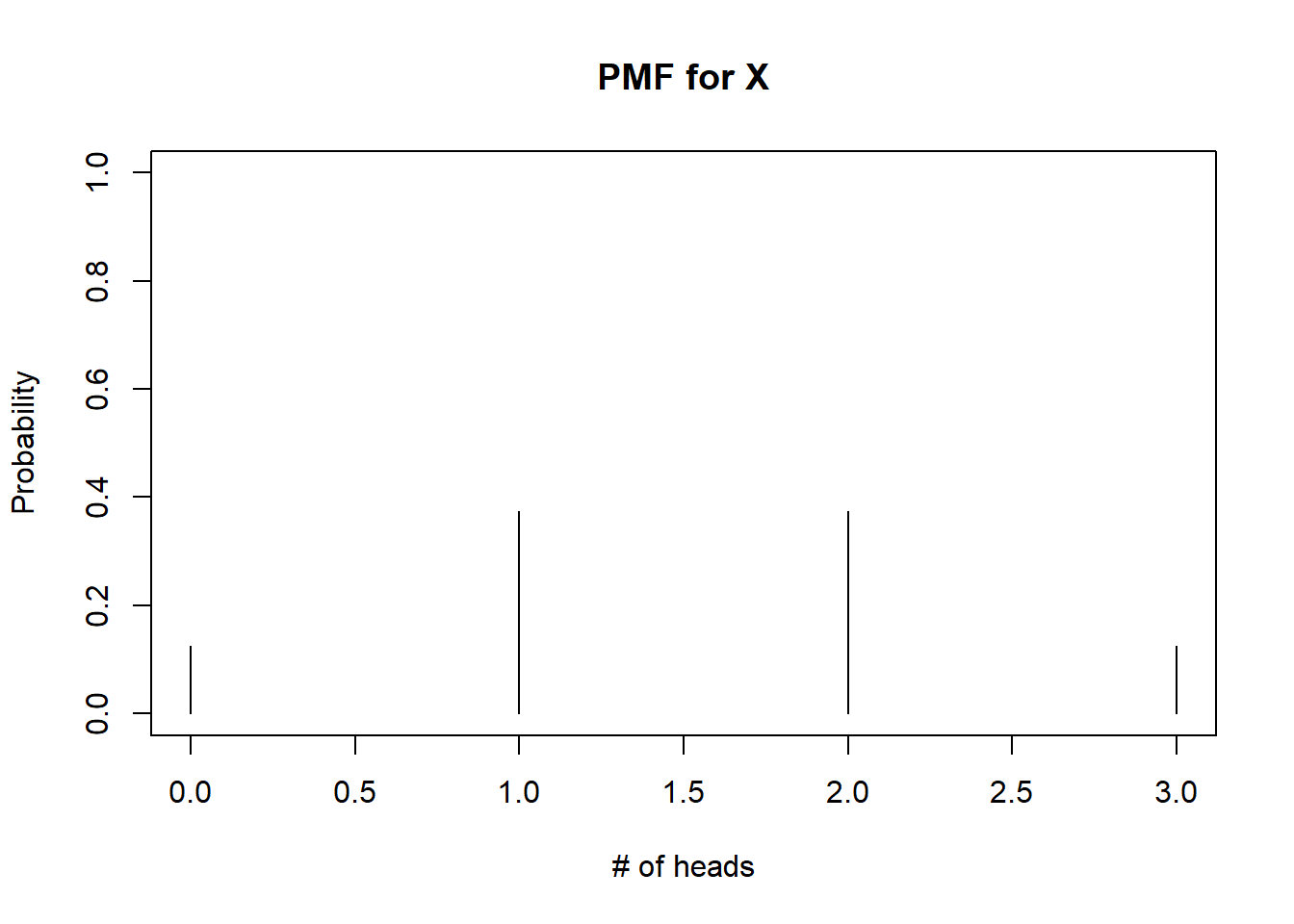

Figure 3.1: PMF for X

The PMF provides a list of all possible values for the random variable and the corresponding probabilities. In other words, the PMF describes the distribution of the relative frequencies for each outcome. For our experiment, observing 1 or 2 heads is equally likely, and they occur three times as often as observing 0 or 3 heads. Observing 0 or 3 heads is also equally likely.

3.2.1 Valid PMFs

Consider a discrete random variable $X$ with support $x_1, x_2, \cdots$. The PMF $P_X(x)$ of $X$ must satisfy:

$P_X(x) > 0$ if $x = x_j$, and $P_X(x) = 0$ otherwise.
$\sum_{j=1}^{\infty} P_X(x_j) = 1$.

In other words, the probabilities associated with the support are greater than 0, and the sum of the probabilities across the whole support must add up to 1.

Thought question: based on Table 3.1, can you see why our PMF for $X$ is valid?

3.2.2 PMFs and Histograms

Recall the frequentist viewpoint of probability, that it represents the relative frequency associated with an event that is repeated for an infinite number of times.

Consider our experiment where we flip a coin 3 times and count the number of heads. The support of our random variable $X$, the number of heads, is $\{0,1,2,3 \}$. Imagine performing our experiment a large number of times. Each time we perform the experiment, we record the number of heads. If we performed the experiment one million times, we would have recorded one million values for the number of heads, and each value must be in the support of $X$. If we then create a histogram for the one million values for the number of heads, the shape of the histogram should be very close to the shape of the plot of the PMF in Figure 3.1. Figure 3.2 below shows the resulting histogram after performing the experiment 1 million times.

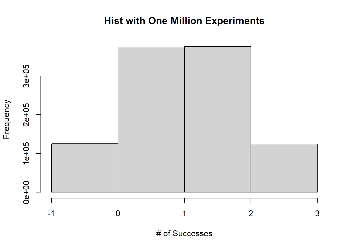
Figure 3.2: Histogram from Experiment Performed 1 Million Times

In general, the PMF of a random variable should match the histogram in the long run.

Note: What we have just done here was to use simulations to repeat an experiment a large number of times.

3.3 Cumulative Distribution Functions (CDFs)

Another function that is used to describe the distribution of discrete random variables is the cumulative distribution function (CDF). The CDF of a random variable $X$ is $F_X(x) = P(X \leq x)$. Notice that unlike the PMF, the definition of CDF applies for both discrete and continuous random variables.

Going back to our example where we record the number of heads out of 3 coin flips, we can write out the CDF for the random variable $X$:

$F_X(0) = P(X \leq 0) = P(X=0) = \frac{1}{8}$,
$F_X(1) = P(X \leq 1) = P(X=0) + P(X=1) = \frac{1}{8} + \frac{3}{8} = \frac{1}{2}$,
$F_X(2) = P(X \leq 2) = P(X=0) + P(X=1) + P(X=2) = \frac{1}{2} + \frac{3}{8} = \frac{7}{8}$,
$F_X(3) = P(X \leq 3) = P(X=0) + P(X=1) + P(X=2) + P(X=3) = \frac{7}{8} + \frac{1}{8} = 1$.

Notice how these calculations were based on the PMF. To find $P(X \leq x)$, we summed the PDF over all values of the support that is less than or equal to $x$. Therefore, another way to write the CDF for a discrete random variable is

\[\begin{equation} F_X(x) = P(X \leq x) = \sum_{x_j \leq x} P(X=x_j). \tag{3.1} \end{equation}\]

Fairly often, the CDF of a discrete random variable is presented in a simple table like Table 3.2 below:

Table 3.2: CDF for X
x	CDF
0	0.125
1	0.500
2	0.875
3	1.000

Or in a simple plot like in Figure 3.3 below:

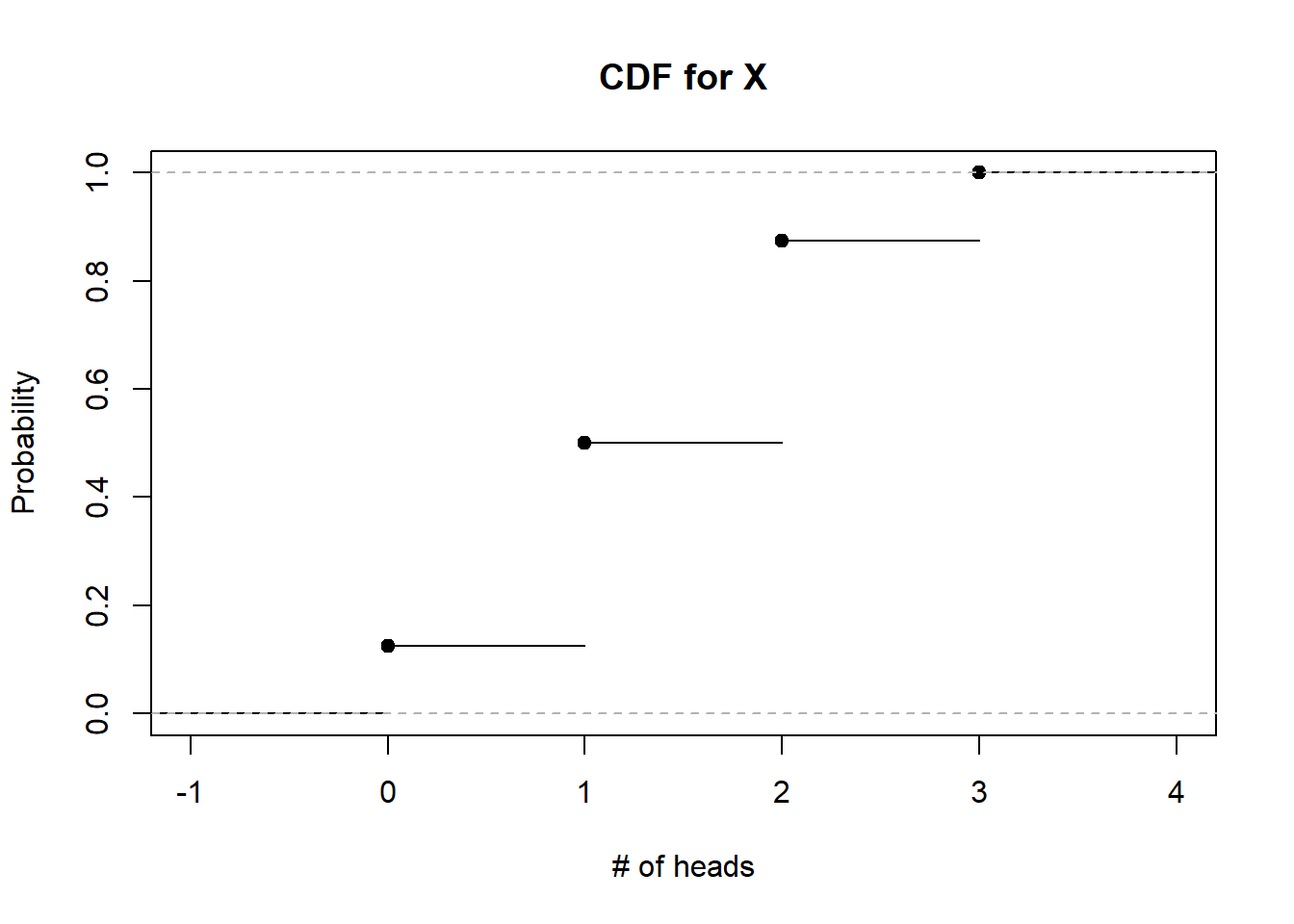
Figure 3.3: CDF for X

The CDF for discrete random variables always look like a step function, as it increases in discrete jumps at each value of the support. The height of each jump corresponds to the PMF at that value of the support.

Thought question: do you see similarities between the CDF and the empirical cumulative density function (ECDF) from section 1.3.3?

3.3.1 Valid CDFs

The CDF $F_X(x)$ of $X$ must:

be non decreasing. This means that as $x$ gets larger, the CDF either stays the same or increases. Visually, a graph of the CDF never decreases as $x$ increases.
approach 1 as $x$ approaches infinity and approach 0 as $x$ approaches negative infinity. Visually, a graph of the CDF should be equal to or close to 1 for large values of x, and it should be equal to or close to 0 for small values of x.

Thought question: Look at the CDF for our example in Figure 3.3, and see how it satisfies the criteria listed above for a valid CDF.

3.4 Expectations

In the previous section, we see how PMFs and CDFs can be used to describe the distribution of a random variable. As the PMF can be viewed as a long-run version of the histogram, it gives us an idea about the shape of the distribution. Similar to Section 1, we will also be interested in measures of centrality and spread for random variables.

A measure of centrality for random variables is the expectation, or expected value. The expectation of a random variable can be interpreted as the long-run mean of the random variable, i.e. if we were able to repeat the experiment an infinite number of times, the expectation of the random variable will be the average result among all the experiments.

For a discrete random variable $X$ with support $x_1, x_2, \cdots,$, the expected value, denoted by $E(X)$, is

\[\begin{equation} E(X) = \sum_{j=1}^{\infty} x_j P(X=x_j). \tag{3.2} \end{equation}\]

We can use Table 3.1 as an example. To find the expected number of heads out of 3 coin flips, using equation (3.2),

\[ \begin{split} E(X) &= 0 \times \frac{1}{8} + 1 \times \frac{3}{8} + 2 \times \frac{3}{8} + 3 \times \frac{1}{8}\\ &= 1.5 \end{split} \]

What we did was to take the product of each value in the support of the random variable with its corresponding probability, and add all these products.

We can see another interpretation of the expected value of a random variable from this calculation: it is the weighted average of the values for the random variable, weighted by their probabilities.

Intuitively, this expected value of 1.5 should make sense. If we flip a coin 3 times, and the coin is fair, we expect half of these flips to land heads, or 1.5 flips to land heads.

View the video below for a more detailed explanation on how to calculate expected values:

3.4.1 Linearity of Expectations

We have seen how to calculate the expected value of a random variable $X$ using equation (3.2). What we need is the PMF of $X$. Sometimes our random variable can be viewed as a sum (or difference) of other random variables, or it could involve a multiplication and / or adding a constant to the random variable. Consider some of these scenarios:

Suppose my friend and I are fisherman. Let $Y$ be the random variable describing the number of fish I catch on a workday, and let $W$ be the random variable describing the number of fish my friend catches on a workday. We can let $T = Y+W$ be the random variable describing the total number of fish we catch on a workday.
Suppose that I sell each fish for $10 and my friend sells each fish for $15. We can let $R = 10Y + 15W$ be the random variable that describes the revenue we generate on a workday.
Suppose that my friend and I rent out a space at the market to sell our fish, and it costs $5 a day to rent out the space. We can let $G = 10Y + 15W - 5$ be the random variable that describes our gross income for the day.

All of these examples involve new random variables, $T, R, G$ that can be based on previously defined random variables, $Y, W$. It turns out that to find the expectations of the new random variables, all we need is the expectations of the previously defined random variables. We do not need to find the PMFs for $T, R$ and $S$ and then apply equation (3.2).

These can be done through the linearity of expectations: Let $X$ and $Y$ denote random variables, and $a,b,c$ denote some constants, then

\[\begin{equation} E(aX + bY + c) = aE(X) + bE(Y) + c. \tag{3.3} \end{equation}\]

Applying equation (3.3) to the fishing examples:

$E(T) = R(Y + W) = E(Y) + E(W)$,
$E(R) = E(10Y + 15W) = 10E(Y) + 15E(W)$,
$E(G) = E(10Y + 15W - 5) = 10E(Y) + 15E(W) - 5$.

All we need to find the expected values for the total number of fish, revenue generated, and gross income were the expected values for the number of fish each of us caught. We do not need the PMFs for $T,R,G$.

3.4.1.1 Visual Explanation

For a visual explanation of why equation (3.3) makes sense, we go back to our previous example where $X$ denotes the number of heads in 3 coin flips. Figure 3.1 displays the PMF for this random variable. Let us create the PMF for a new random variable $Y=2X$ and display it in Figure 3.4 below:

##support of X
x<-0:3
## PMF for each value in the support. 
PMFs<-c(1/8, 3/8, 3/8, 1/8)
EX<-1.5

##support of Y
y<-2*x
## PMF for each value in the support. 
PMFs<-c(1/8, 3/8, 3/8, 1/8)
EY<-2*EX

par(mfrow=c(2,1))

## create plot of PMF vs each value in support
plot(x, PMFs, type="h", main = "PMF for X", xlab="X", ylab="Probability", ylim=c(0,1))
##overlay a line representing EX in red
abline(v=EX, col="red")

## create plot of PMF vs each value in support
plot(y, PMFs, type="h", main = "PMF for Y", xlab="Y", ylab="Probability", ylim=c(0,1))
##overlay a line representing EY in red
abline(v=EY, col="red")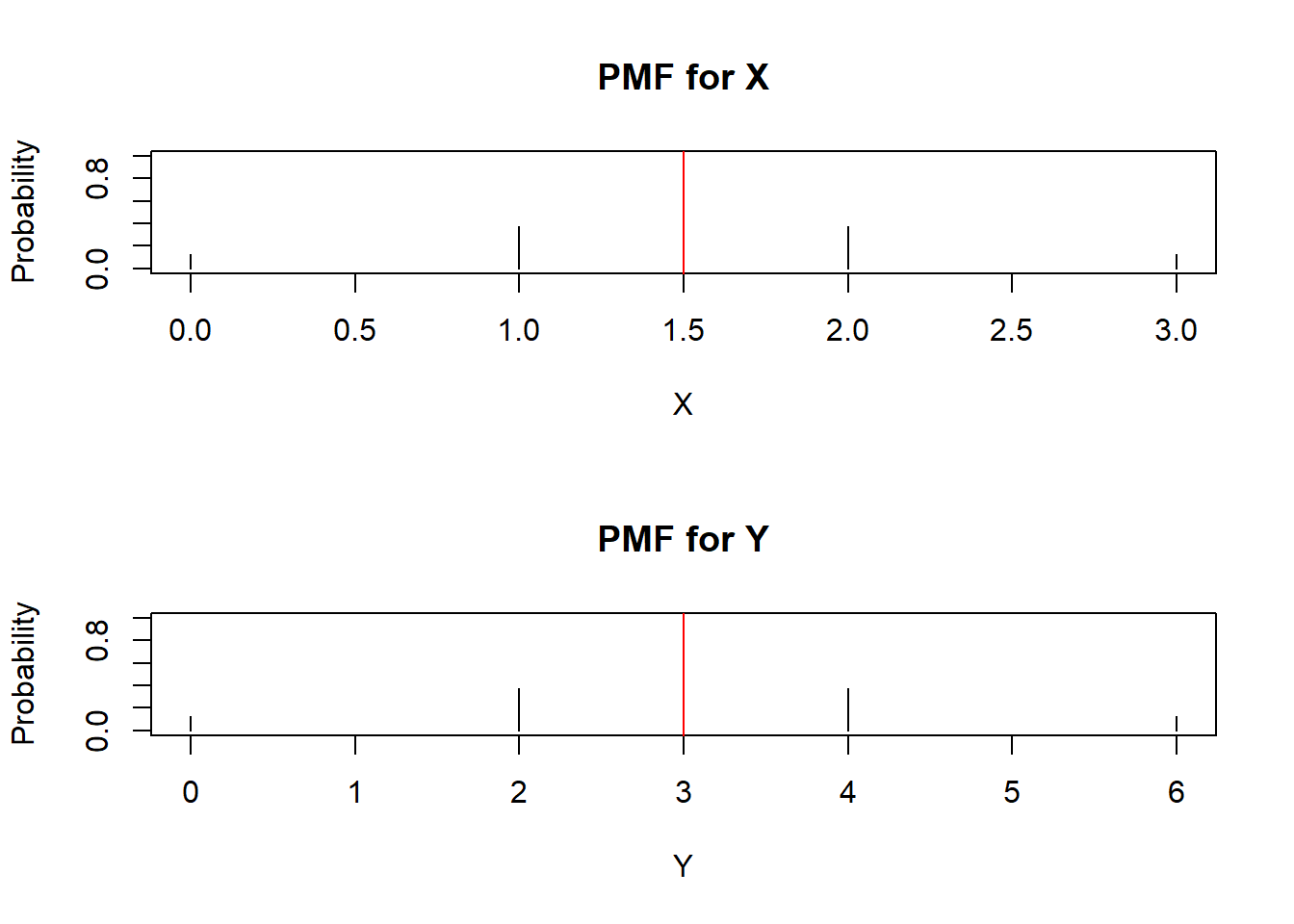

Figure 3.4: PMF for X and Y=2X

Note that the red vertical lines represent the expected value for the random variable, and since the PMFs are symmetric, the expected value lies right in the middle of the support. Comparing the PMFs in Figure 3.4, we get $Y$ by multiplying $X$ by 2. So the support of $Y$ is now $\{0,2,4,6\}$ but the associated probabilities are unchanged, so the heights of the probabilities on the vertical axis are unchanged. Therefore, the center, the expected value, is multiplied by the same constant.

Consider another random variable $W = X+3$. We create the PMF for $W$ and display it in Figure 3.5 below:

##support of X
x<-0:3
## PMF for each value in the support. 
PMFs<-c(1/8, 3/8, 3/8, 1/8)
EX<-1.5

##support of W
w<-x+3
## PMF for each value in the support. 
PMFs<-c(1/8, 3/8, 3/8, 1/8)
EW<-EX+3

par(mfrow=c(2,1))

## create plot of PMF vs each value in support
plot(x, PMFs, type="h", main = "PMF for X", xlab="X", ylab="Probability", ylim=c(0,1))
##overlay a line representing EX in red
abline(v=EX, col="red")

## create plot of PMF vs each value in support
plot(w, PMFs, type="h", main = "PMF for w", xlab="W", ylab="Probability", ylim=c(0,1))
##overlay a line representing EW in red
abline(v=EW, col="red")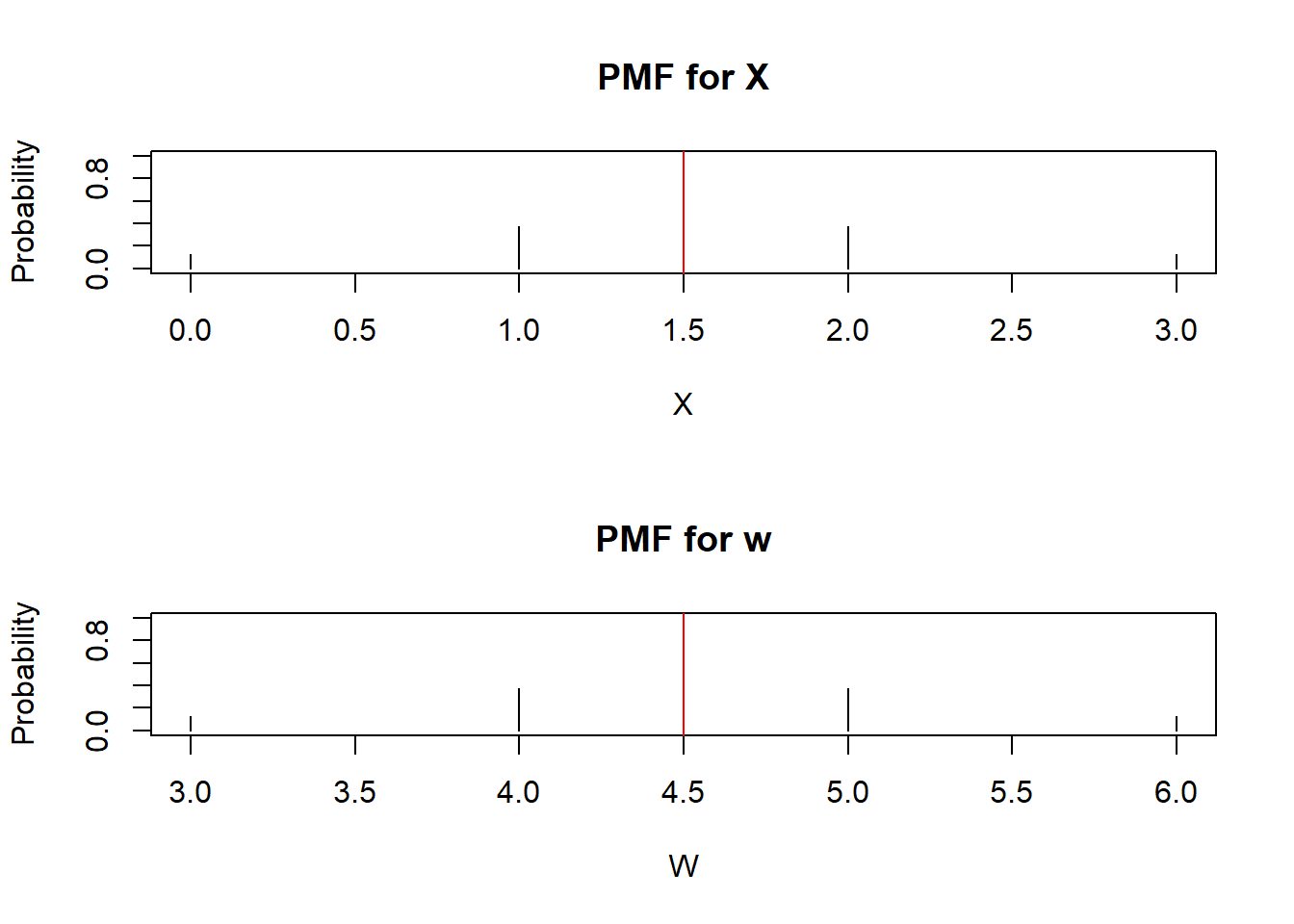

Figure 3.5: PMF for X and W=X+3

Notice the PMFs for $X$ and $W$ look almost exactly the same. The only difference is that every value in the support for $X$ is shifted by 3 units. The probabilities stay the same, so the heights in the PMFs are unchanged. So if every value is shifted by 3 units, the expected value, the long-run average, also gets shifted by 3 units. Adding a constant to a random variable shifts the expected value accordingly.

3.4.1.2 One More Example

We look at one more example to illustrate the usefulness of the linearity of expectations. Consider a drunk man who has to walk on a one-dimensional number line and starts at the 0 position. For each step the drunk man takes, he either moves forward, backward, or stays at the same spot. He steps forward with probability $p_f$, backward with probability $p_b$, and stays at the same spot with probability $p_s$, where $p_f + p_b+p_s = 1$. Let $Y$ be the position on the number line of the drunk man after 2 steps. What is the expected position of the drunk man after two steps, i.e. what is $E(Y)$? Assume that each step is independent.

Using brute force, we can find the PMF of $Y$, and find $E(Y)$ using equation (3.2). First, we need to find the sample space for $Y$. With two steps, the sample space is $\{-2,-1,0,1,2\}$. Next, we need to find the probabilities associated with each outcome in the sample space.

For $Y=-2$, the man must move backward on each step. This probability will be $P(Y=-2) = p_b^2$.
Likewise, for $Y=2$, the man must move forward on each step. This probability will be $P(Y=2) = p_f^2$.
For $Y=-1$, the man could stay on the first step, then move back on the second, or move back on the first step, and stay on the second. This probability will be $P(Y=-1) = p_s p_b + p_b p_s = 2p_b p_s$.
Likewise, for $Y=1$, the man could stay on the first step, then move forward on the second, or move forward on the first step, and stay on the second. This probability will be $P(Y=1) = p_s p_f + p_f p_s = 2p_f p_s$.
For $Y=0$, the man could move forward, then backward, or move backward then forward, or stay on both steps. So $P(Y=0) = p_f p_b + p_b p_f + p_s^2 = p_s^2 + 2 p_b p_f$.

Using equation (3.2),

\[ \begin{split} E(Y) &= -2 \times p_b^2 + -1 \times 2p_b p_s + 0 \times p_s^2 + 2 p_b p_f + 1 \times 2p_f p_s + 2 \times p_f^2 \\ &= 2 (p_f - p_b) \end{split} \]

Note: I skipped a lot of messy algebra to get to the end result. Even with skipping some of the messy algebra, setting up the PMF was quite a bit of work.

Suppose we use the linearity of expectations in equation (3.3). Let $Y_1, Y_2$ denote the distance the man moves at step 1 and 2 respectively. Then $Y = Y_1 + Y_2$. The sample of $Y_1$ and $Y_2$ are the same: $\{-1,0,1\}$. Both $Y_1$ and $Y_2$ have the following PMF:

$P(Y_i = -1) = p_b$
$P(Y_i = 0) = p_s$
$P(Y_i = 1) = p_f$

And using equation (3.2),

\[ \begin{split} E(Y_i) &= -1 \times p_b + 0 \times p_s + 1 \times p_f \\ &= p_f - p_b \end{split} \]

So therefore $E(Y) = E(Y_1 + Y_2) = E(Y_1) + E(Y_2) = 2(p_f - p_b)$. Both approaches resulted in the same answer, but notice how much simpler its was to obtain the solution using linearity of expectations. Imagine if we wanted to find the expected position after 500 steps? Writing out the sample space for 500 steps will be extremely long.

View the video below for a more detailed explanation of this worked example:

3.4.2 Law of the Unconscious Statistician

Suppose we have the PMF of a random variable $X$, and we want to find $E(g(X))$, where $g$ is a function of $X$ (you can think of $g$ as a transformation performed on $X$). One idea could be to find the PMF of $g(X)$ and then use the definition of expectation in equation (3.2). But we have seen in the previous subsection that finding the sample space after transforming the random variable can be challenging. It turns out we can find $E(g(X))$ based on the PMF of $X$, without having to find the PMF of $g(X)$.

This is done through the Law of the Unconscious Statistician (LOTUS). Let $X$ be a discrete random variable with support $\{x_1, x_2, \cdots \}$, and $g$ is a function applied to $X$, then

\[\begin{equation} E(g(X)) = \sum_{i=j}^{\infty} g(x_j) P(X=x_j). \tag{3.4} \end{equation}\]

An application of LOTUS is in finding the variance of a discrete random variable.

3.4.3 Variance

We have talked about the shape of the distribution of a discrete random variable, and its expected value. One more measure that we are interested in is the spread associated with the distribution. One common measure is the variance of the random variable.

The variance of a random variable $X$ is

\[\begin{equation} Var(X) = E[(X - EX)^2] \tag{3.5} \end{equation}\]

and the standard deviation of a random variable $X$ is the square root of its variance

\[\begin{equation} SD(X) = \sqrt{Var(X)}. \tag{3.6} \end{equation}\]

Looking at equation (3.5) a little more closely, we can see a natural interpretation of the variance of a random variable: it is the average squared distance of the random variable from its mean, in the long-run. An equivalent formula for the variance of a random variable is

\[\begin{equation} Var(X) = E(X^2) - (EX)^2. \tag{3.7} \end{equation}\]

Equation (3.7) is easier to work with than equation (3.5) when performing actual calculations.

Let us now go back to our original example, where $X$ denotes the number of heads out of 3 coin flips. Earlier, we found the PMF of this random variable, per Table 3.1, and we found its expectation to be 1.5. To find the variance of $X$ using equation (3.7), we find $E(X^2)$ first using LOTUS in equation (3.4)

\[ \begin{split} E(X^2) &= 0^2 \times \frac{1}{8} + 1^2 \times \frac{3}{8} + 2^2 \times \frac{3}{8} + 3^2 \times \frac{1}{8} \\ &= 3 \end{split} \]

so $Var(x) = 3 - 1.5^2 = \frac{3}{4}$.

Thought question: Try to find $Var(X)$ using equation (3.5) and LOTUS. You should arrive at the same answer but the steps may be a bit more complicated.

View the video below for a more detailed explanation on how to calculate variance of discrete random variables using equations (3.7) and (3.5):

3.4.3.1 Properties of Variance

Variance has the following properties:

$Var(X+c) = Var(X)$, where $c$ is a constant. This should make sense, since if we add a constant to a random variable, we shift it by $c$ units. As shown earlier in Figure 3.5, the expected value also gets shifted by $c$ units. Variance measures the average squared distance of a variable from its mean. So the distance, and the squared distance, of $X$ from its mean is unchanged.
$Var(cX) = c^2 Var(X)$. Look at Figure 3.4, notice the distance between each value in the support from its expected value gets multiplied by 2 (since $Y=2X$). So if we multiply a random variable by $c$, the distance between each value in the support on its expected value is multiplied by $c$. Since variance measures squared distance, the variance gets multiplied by $c^2$.
If $X$ and $Y$ are independent random variables, then $Var(X+Y) = Var(X) + Var(Y)$.

3.5 Common Discrete Random Variables

Next, we will introduce some commonly used distributions that may be used for discrete random variables. A number of common statistical models (for example, logistic regression, Poisson regression) are based on these distributions.

3.5.1 Bernoulli

The Bernoulli distribution might be the simplest discrete random variable. The support for such a random variable is $\{0,1\}$. In other words, the value of a random variable that follows a Bernoulli distribution is either 0 or 1. A Bernoulli distribution is also described by the parameter $p$, which is the probability that the random variable takes on the value of 1.

More formally, a random variable $X$ follows a Bernoulli distribution with parameter $p$ if $P(X=1) = p$ and $P(X=0) = 1-p$, where $0<p<1$. Using mathematical notation, we can write $X \sim Bern(p)$ to express that the random variable $X$ is distributed as a Bernoulli with parameter $p$. The PMF of a Bernoulli distribution is written as

\[\begin{equation} P(X=k) = p^k (1-p)^{1-k} \tag{3.8} \end{equation}\]

for $k=0, 1$.

It is not enough to specify that a random variable follows a Bernoulli distribution. We need to also clearly specify the value of the parameter $p$. Consider the following two examples which describe two different experiments:

Suppose I flip a fair coin once. Let $Y=1$ if the coin lands heads, and $Y=0$ if the coin lands tails. $Y \sim Bern(\frac{1}{2})$ in this example since the coin is fair.
Suppose I am asked a question and I am given 5 multiple choices, of which only 1 is the correct answer. I have no idea about the topic, and the multiple choices do not help, so I have to guess. Let $W=1$ if I answer correctly, and $W=0$ if I answer incorrectly. $W \sim Bern(\frac{1}{5})$.

$P(Y=1)$ and $P(W=1)$ are not the same in these examples.

Fairly often, when we have a Bernoulli random variable, the event that results in the random variable being coded as 1 is called a success, and the event that results in the random variable being coded as 0 is called a failure. In such a setting, the parameter $p$ is called the success probability of the Bernoulli distribution. An experiment that has a Bernoulli distribution can be called a Bernoulli trial.

If you go back to the second example in section ??, we were modeling whether a job applicant receives a callback or not. In this example, we could let $V$ be the random variable that an applicant receives a callback, with $V=1$ denoting the applicant received a callback, and $V=0$ when the applicant did not receive a callback. We used logistic regression in the example. It turns out that logistic regression is used when the variable of interest follows a Bernoulli distribution.

3.5.1.1 Properties of Bernoulli

Consider $X$ is a Bernoulli distribution with parameter $p$. The expectation of a Bernoulli distribution is

\[\begin{equation} E(X) = p \tag{3.9} \end{equation}\]

and its variance is

\[\begin{equation} Var(X) = p(1-p). \tag{3.10} \end{equation}\]

Thought question: Use the definition of expectations for discrete random variables, equation (3.2), and the PMF of a Bernoulli random variable, and LOTUS to prove equations (3.9) and (3.10).

The expected value being equal to $p$ for a Bernoulli distribution should make sense. Remember that the support for such a random variable is 0 or 1, with $P(X=1) = p$. Using the frequentist viewpoint, if we were to flip a coin and record heads or tails, and repeat this coin flipping many times, we will have record a bunch of 0s and 1s to represent the result for all the coin flips. The average of this bunch of 0s and 1s is just the proportion of 1s.

The equation for the variance of a Bernoulli distribution exhibits an interesting and intuitive behavior. Figure 3.6 below shows how the variance behaves as we vary the value of $p$:

p<-seq(0,1,by = 0.001) ##sequence of values for p
Bern_var<-p*(1-p) ##variance of Bernoulli
##plot variance against p
plot(p, Bern_var, ylab="Variance", main="Variance of Bernoulli as p is Varied")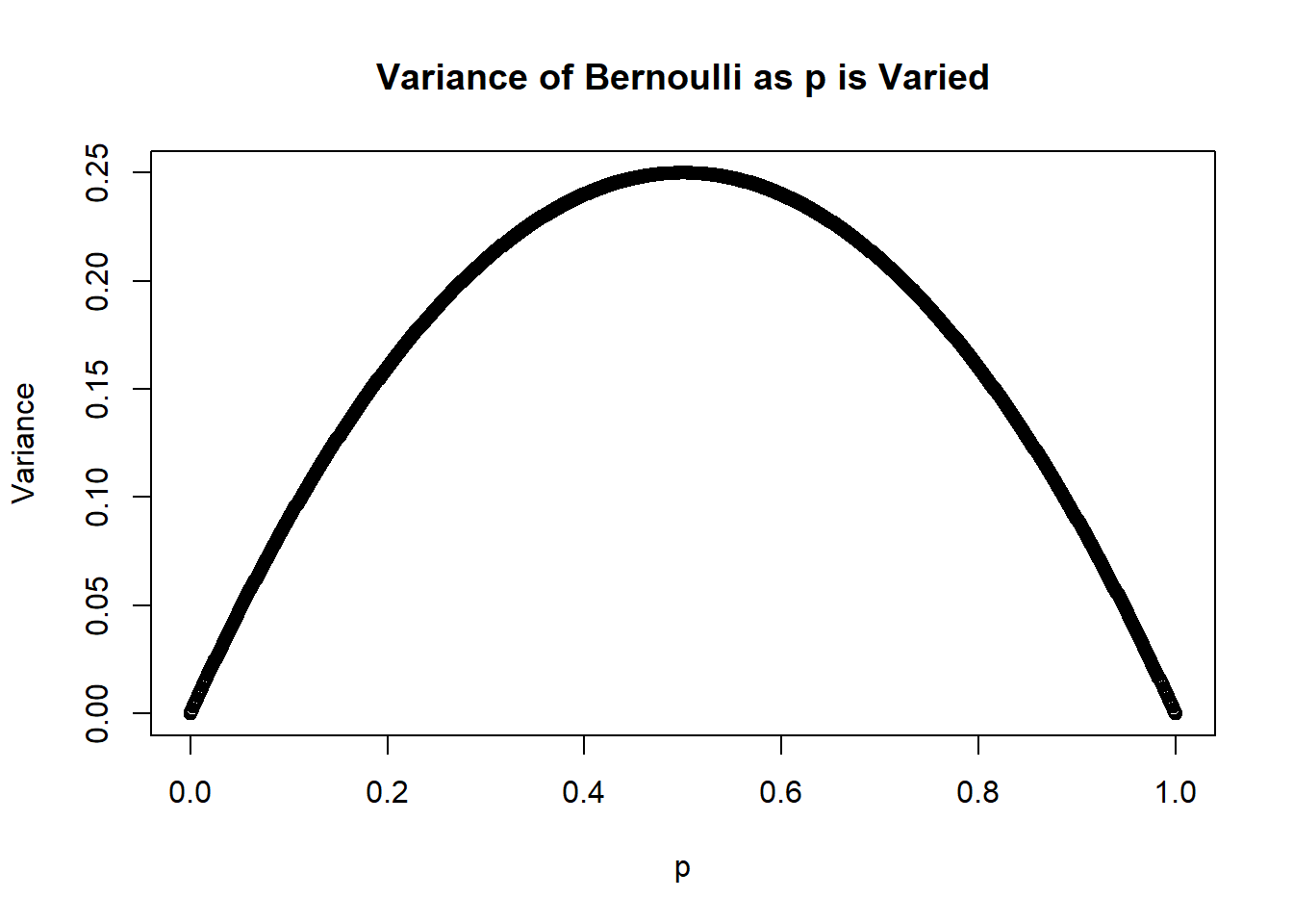

Figure 3.6: Variance of Bernoulli

Notice the variance is at a maximum when $p=0.5$, and the variance is minimum (in fact it is 0) when $p=0$ or $p=1$. If we have a biased coin such that it always lands heads, every coin flip will land on heads with no exception. There is no variability in the result, and we have utmost certainty in the result of each coin flip. On the other hand, if the coin is fair such that $p=0.5$, we have the least certainty in the result of each coin flip, and so variance is maximum when the coin is fair.

Another application of this property is during election results (assuming 2 candidates, but the same idea applies for more candidates). For swing states where the race is closer (so $p$ is closer to half), projections on the winner have more uncertainty and so we need to get more data and wait longer for the projections. For states that primarily vote for one candidate (so $p$ is closer to 0 or 1), projections happen a lot quicker as projections have less uncertainty.

3.5.2 Binomial

Suppose we have an experiment that follows a Bernoulli distribution, and we perform this experiment $n$ times (sometimes called trials), each time with the same success probability $p$. The experiments are independent from each other. Let $X$ denote the number of successes out of the $n$ trials. $X$ follows a binomial distribution with parameters $n$ and $p$ (number of trials and success probability). We write $X \sim Bin(n,p)$ to express that $X$ follows a binomial distribution with parameters $n$ and $p$, with $n>0$ and $0<p<1$. The PMF of a Binomial distribution is written as

\[\begin{equation} P(X=k) = \binom{n}{k} p^k (1-p)^{n-k} \tag{3.11} \end{equation}\]

for $k=0,1,2, \cdots, n$, which is also the support of the binomial distribution.

In equation (3.11), $\binom{n}{k}$ is called the binomial coefficient, and it is the number of combinations that result in $k$ successes out of the $n$ trials. The binomial coefficient can be found using

\[\begin{equation} \binom{n}{k} = \frac{n!}{k! (n-k)!}. \tag{3.12} \end{equation}\]

$n!$ is called n-factorial, and is the product of all positive integers less than or equal to n. So $n! = n \times (n-1) \times (n-2) \times \cdots \times 1.$ As an example $5! = 5 \times 4 \times 3 \times 2 \times 1 = 120$, or using R:

factorial(5)

## [1] 120

Note: A fairly common model, the logistic regression model with aggregated data, is based on the binomial distribution. We mentioned logistic regression earlier. The difference between these two (with and without aggregated data) is based on the structure of the data frame. If you are interested in these differences, please read https://www.r-bloggers.com/2021/02/how-to-run-logistic-regression-on-aggregate-data-in-r/.

We go back to our first example of counting the number of heads out of three coin flips follows a binomial distribution.

Each coin flip is either heads or tails. There are only two outcomes for each flip.
The success probability, the probability of heads, is 0.5 and is the same for each flip. The parameter is fixed for each flip.
The result of each flip is independent of other flips since other flips do not affect the outcome.
The number of trials (flips in this example) is $n=3$ is specified as a fixed value.

Since these four conditions are met, the number of heads in 3 coin flips can be modeled using a binomial distribution. We let $x$ denote the number of heads in 3 coin clips, so we write $X \sim Bin(3,0.5)$.

Suppose we want to calculate $P(X=2)$ using equation (3.11):

\[ \begin{split} P(X=2) &= \binom{3}{2} (0.5)^2 (0.5)^1\\ &= \frac{3!}{2! 1!} (0.5)^2 (0.5)^1 \\ &= 3 \times \frac{1}{8} \\ &= \frac{3}{8}. \end{split} \]

In this example, the binomial coefficient equals to 3. Which indicates there were 3 combinations to obtain 2 heads in 3 coin flips. $P(X=2)$ can be written as $P(HHT \cup HTH \cup THH)$. Solving for $P(HHT \cup HTH \cup THH)$, we have

\[ \begin{split} P(HHT \cup HTH \cup THH) &= P(HHT) + P(HTH) + P(THH)\\ &= 0.5^3 + 0.5^3 + 0.5^3 \\ &= 3 \times \frac{1}{8} \\ &= \frac{3}{8}. \end{split} \] so we could have solved this using basic probability rules from the previous module, without using the PMF of the binomial distribution in equation (3.11). Of course, the PMF of the binomial distribution gets a lot more convenient if $n$ gets larger, as the number of combinations and sample space get a lot larger.

We can also use R to find $P(X=2)$:

dbinom(2,3,0.5) ##specify values of k, n, p in this order

## [1] 0.375

3.5.2.1 Relationship Between Binomial and Bernoulli

Looking at the description of the Bernoulli and binomial distributions, you may notice that a Bernoulli random variable is a special case of a binomial random variable when $n=1$, i.e. when we have only 1 trial.

The binomial random variable is also sometimes viewed as the sum of $n$ independent Bernoulli random variables, all with the same value of $p$.

3.5.2.2 Properties of Binomial

If $X \sim Bin(n,p)$, then

\[\begin{equation} E(X) = np \tag{3.13} \end{equation}\]

and

\[\begin{equation} Var(X) = np(1-p). \tag{3.14} \end{equation}\]

These results should make sense when we note the relationship between a binomial random variable and Bernoulli random variable. Suppose we have random variables $Y_1, Y_2, \cdots, Y_n$ and they are all Bernoulli random variables with parameter $p$ and are independent. Then $Y = Y_1 + Y_2 + \cdots + Y_n \sim Bin(n,p)$. Therefore, using the linearity of expectations in equation (3.3), $E(Y) = E(Y_1) + E(Y_2) + \cdots + E(Y_n) = np$. Since $Y_1, Y_2, \cdots, Y_n$ are independent, $Var(Y) = Var(Y_1) + Var(Y_2) + \cdots + Var(Y_n) = np(1-p)$.

3.5.2.3 PMFs of Binomial

We take a look at the PMFs of a few binomials, all with $n=10$ but we vary $p$ to be 0.2, 0.5, and 0.9, in Figure 3.7:

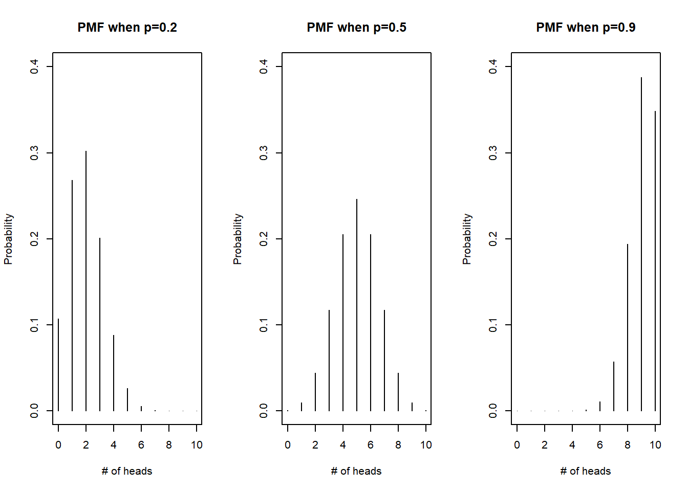
Figure 3.7: PMF for X, n=10, p varied

From figure 3.7, we can see that the distribution of the binomial is symmetric when $p=0.5$, as middle values of $k$ have higher probabilities, and the probabilities decrease as we go further away from the middle. When $p \neq 0.5$, we see that the distribution gets skewed. When the success probability is small, smaller number of successes are likelier, and when the success probability is large, larger number of successes are likelier, which is intuitive. If the probability of success is small, we expect most outcomes to be failures.

3.5.3 Poisson

One more common distribution used for discrete random variables is the Poisson distribution. This is often used when the variable of interest is what we call count data (the support is non negative integers), for example, the number of cars that cross an intersection during the day.

A random variable $X$ follows a Poisson distribution with parameter $\lambda$, where $\lambda>0$. Using mathematical notation, we can write $X \sim Pois(\lambda)$ to express that the random variable $X$ is distributed as a Poisson with parameter $p$. The PMF of a Poisson distribution is written as

\[\begin{equation} P(X=k) = \frac{e^{-\lambda}\lambda^k}{k!} \tag{3.15} \end{equation}\]

for $k=0,1,2,\cdots$. $\lambda$ is sometimes called a rate parameter, as it is related to the rate of arrivals, for example, the number of that cross an intersection during a period of time.

3.5.3.1 Properties of Poisson

If $X \sim Pois(\lambda)$, then

\[\begin{equation} E(X) = \lambda \tag{3.16} \end{equation}\]

and

\[\begin{equation} Var(X) = \lambda. \tag{3.17} \end{equation}\]

These imply that larger values of a Poisson random variable are associated with larger variances. This is a common feature for count data. Consider the number of cars that cross an intersection during a one-hour time period. Consider the average number of cars during rush hour, say between 5 and 6pm. This average number is large, but the number could be a lot smaller due to inclement weather, or the number could get a lot larger is there is a convention occurring nearby. On the other hand, consider the average number of cars between 3 and 4am. This average number is small, and is likely to be small all the time, regardless of weather conditions and whether special events are happening.

Another interesting property of the Poisson distribution is that it is skewed when $\lambda$ is small, and approaches a bell-shaped distribution as $\lambda$ gets bigger. Figure 3.8 displays density plots of Poisson distributions as $\lambda$ is varied:

##calculate probability of Poisson with these values on the support
x<-0:20
lambda<-c(0.5, 1, 4, 10) ##try 4 different values of lambda

##create PMFs of these 4 Poissons with different lambdas
par(mfrow=c(2,2))
for (i in 1:4)
  
{
  dens<-dpois(x,lambda[i])
  plot(x, dens, type="l", main=paste("Lambda is", lambda[i]))
}

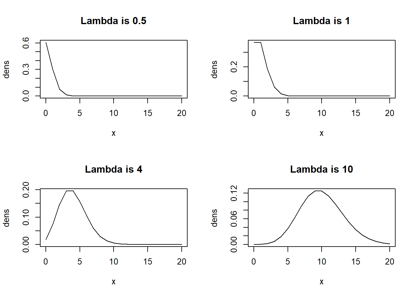
Figure 3.8: PMF for Poissons as Rate Parameter is Varied

3.5.3.2 Poisson Approximation to Binomial

If $X \sim Bin(n,p)$, and if $n$ is large and $p$ is small, then the PMF of $X$ can be approximated by a Poisson distribution with rate parameter $\lambda = np$. In other words, the approximation works better as $n$ gets larger and $np$ gets smaller.

There are several rules of thumbs that exist to guide as to how large $n$ should be and how small $np$ should be. The National Institute of Standards and Technology (NIST) suggest $n \geq 20$ and $p \leq 0.05$, or $n \geq 100$, and $np \leq 10$.

One of the main for using this approximation, instead of directly using the binomial distribution, is that the binomial coefficient can become computationally expensive to compute when $n$ is large.

Consider this example: A company manufactures computer chips, and 2 percent of chips are defective. The quality control manager randomly samples 100 chips coming off the assembly line. What is the probability that at most 3 chips are defective?

Let $Y$ denote the number of chips that are defective out of 100 chips.

Each chip is either defective or not. There are only two outcomes for each chip.
The “success” probability is 0.02 for each chip. This probability is assumed to be fixed for each chip.
We have to assume that each chip is independent.
The number of chips is fixed at $n=100$.

So we can model $Y \sim Bin(100,0.02)$, as long as we assume the chips the independent. To find $P(Y \leq 3)$, we can:

use the binomial distribution, or
approximate it using $Pois(2)$, as $\lambda = np = 100 \times 0.02$.

##set up binomial
n<-100 
p<-0.02 
y<-0:3 ##we want P(Y=0), P(Y=1), P(Y=2), P(Y=3)
sum(dbinom(y,n,p))

## [1] 0.8589616

##Use Poisson to approx binomial
lambda<-n*p
sum(dpois(y,lambda))

## [1] 0.8571235

Notice the values are very close to each other.

3.6 Using R

R has built in functions to compute the PMF, CDF, percentiles, as well as simulate data of common distributions. We will start using a random variable $Y$ which follows binomial distribution, with $n=5, p = 0.3$ as an example first. Note in this example that the support for $Y$ is $\{0,1,2,3,4,5 \}$.

To find $P(Y=2)$, use:

dbinom(2, 5, 0.3) ##supply the value of Y you want, then the parameters n and p in this order

## [1] 0.3087

The probability that $Y$ is equal to 2 is 0.3087.

To find $P(Y \leq 2)$, use:

pbinom(2, 5, 0.3) ##supply the value of Y you want, then the parameters n and p in this order

## [1] 0.83692

The probability that $Y$ is less than or equal to 2 is 0.83692.

To find the value on the support that corresponds to the median (or 50th percentile), use:

qbinom(0.5, 5, 0.3) ##supply the value of the percentile you need, then the parameters n and p in this order

## [1] 1

The median of a binomial distribution with 5 trials and success probability 0.3 is 1.

To simulate 10 realizations (replications) of $Y$, use:

set.seed(2) ##use set.seed() so we get the same random numbers each time the code is run
rbinom(10, 5, 0.3) ##supply the number of simulated data you need, then the parameters n and p

##  [1] 1 2 2 0 3 3 0 2 1 2

This outputs a vector of length 10. Each value represents the result of each rep. So the first time we ran the binomial distribution with $n=5, p=0.3$, only 1 out of the 5 was a success. The second time it was run, only 2 out of the 5 was a success, and so on.

Notice these functions all ended with binom. We just added a different letter first, depending on whether we want the PMF, CDF, percentile, or random draw. The letters are d, p, q, and r respectively.

The same idea works for any other distribution. For example, to find the probability of a Poisson distribution with rate parameter 2 being equal to 1, we type:

dpois(1, 2) ##supply value of k, then parameter

## [1] 0.2706706

Thought questions: Suppose $Y \sim Pois(1)$.

Find $P(Y \leq 2)$.
Find the 75th percentile of $Y$.
Simulate 10,000 reps from Y, and find its sample mean. Is the sample mean close to the expected value?

2 Probability

4 Continuous Random Variables