5 Joint Distributions

This module is based on Introduction to Probability (Blitzstein, Hwang), Chapters 7 and 9. You can access the book for free at https://stat110.hsites.harvard.edu/ (and then click on Book). Please note that I cover additional topics, and skip certain topics from the book. You may skip Story 7.1.9, Theorems 7.1.10 to 7.1.12, Examples 7.1.23 to 7.1.26, Section 7.2, Examples 7.3.6 to 7.3.8, 7.4.8 (parts d and f only), Definition 7.5.6, Examples 9.1.8 to 9.1.10, Example 9.2.5, Theorem 9.3.2, Example 9.3.3, Theorems 9.3.7 to 9.3.9, and Sections 9.4 to 9.6 from the book.

5.1 Introduction

In the previous two modules, we learned how to summarize the distribution of individual random variables. We are now ready to extend the concepts from these modules and apply them to a slightly different setting, where we are analyzing how multiple variables are related to each other. It is extremely common to want to analyze the relationship between at least two variables. The book lists a few examples, but here are a few more:

• Public policy: How does increasing expenditure on infrastructure impact economic development?
• Education: How do smaller class sizes and higher teacher pay impact student learning outcomes?
• Marketing: How does the design of a website influence the probability of a customer purchasing an item?

This module will consider these variables jointly, in other words, how they relate to each other. A lot of the concepts such as CDF, PDF, PMF, expectations, variances, and so on will have analogous versions when considering variables jointly.

5.1.1 Module Roadmap

• Section 5.2 will explore these concepts when the variables are discrete. These concepts are easier to learn when the variables are discrete.
• Section 5.3 will introduce these concepts when the variables are continuous.
• Section 5.4 covers a couple of common ways to quantify the strength of the linear relationship between two quantitative variables.
• Section 5.5 covers the notion of the conditional expectation of a random variable.
• Section 5.6 introduces common multivariate distributions.

5.2 Joint Distributions for Discrete RVs

We will start with discrete random variables, then move on to continuous random variables. To keep things simple, we will use two random variables to explain concepts. These concepts can then be generalized to any number of random variables.

Recall that for a single discrete random variable \(X\), we use the PMF to inform us the support of \(X\) and the probability associated with each value of the support. We said that the PMF informs us about the distribution of the random variable \(X\).

We now have two discrete random variables, \(X\) and \(Y\). The joint distribution of \(X\) and \(Y\) provides the probability associated with each possible combination of \(X\) and \(Y\). The joint PMF of \(X\) and \(Y\) is

\[\begin{equation} p_{X,Y}(x,y) = P(X=x, Y=y). \tag{5.1} \end{equation}\]

Equation (5.1) can be read as the probability that the random variables \(X\) and \(Y\) are equal to \(x\) and \(y\) respectively. Recall that upper case letters are usually used to denote random variables, and lower case letters are usually used as a placeholder for an actual numerical value that the random variable could take.

Joint distributions are sometimes called multivariate distributions. If we are looking at the distribution of one random variable, its distribution can be called a univariate distribution.

Joint PMFs can be displayed via a table, like in Table 5.1 below. In this example, we consider how study time, \(X\), is related with grades, \(Y\), with

• \(X=1\) for studying 0 to 5 hours a week,
• \(X=2\) for studying 6 to 10 hours a week, and
• \(X=3\) for studying more than 10 hours a week.
• \(Y=1\) denotes getting an A,
• \(Y=2\) denotes getting a B, and
• \(Y=3\) denotes getting a C or lower.

Table 5.1: Example Joint PMF of Study Time (\(X\)) and Grades (\(Y\))

	X=1	X=2	X=3
Y=1	0.05	0.15	0.30
Y=2	0.05	0.20	0.10
Y=3	0.10	0.05	0

We could also write the joint PMF as:

• \(P(X=1, Y=1) = 0.05\)
• \(P(X=1, Y=2) = 0.05\)
• \(P(X=1, Y=3) = 0.10\)
• \(P(X=2, Y=1) = 0.15\)
• \(P(X=2, Y=2) = 0.20\)
• \(P(X=2, Y=3) = 0.05\)
• \(P(X=3, Y=1) = 0.30\)
• \(P(X=3, Y=2) = 0.10\)
• \(P(X=3, Y=3) = 0\)

Just like the PMFs of a single discrete random variable must sum to 1 and each PMF must be non negative, the joint PMFs of discrete random variables must sum to 1 and each individual PMF must be non negative to be valid.

Thought question: Can you verify that the joint PMF in Table 5.1 is valid?

The joint CDF of any discrete random variables \(X\) and \(Y\) is

\[\begin{equation} F_{X,Y}(x,y) = P(X \leq x, Y \leq y). \tag{5.2} \end{equation}\]

Thought question: Compare equation (5.2) with its univariate counterpart in equation (3.1). Can you see the similarities and differences?

5.2.1 Marginal Distributions for Discrete RVs

From the joint distribution of \(X\) and \(Y\), we can get the distribution of each individual random variable. We call this the marginal distribution, or unconditional distribution, of \(X\) and \(Y\). The marginal distribution of \(X\) gives us information about the distribution of \(X\), without taking \(Y\) into consideration. To get the marginal PMF of \(X\) from the joint PMF of \(X\) and \(Y\):

\[\begin{equation} P(X=x) = \sum_y P(X=x, Y=y). \tag{5.3} \end{equation}\]

Note that the summation is performed over the support of \(Y\). We go back to Table 5.1 as an example. Suppose we want to find the marginal distribution of study times, \(X\). Applying equation (5.3):

\[ \begin{split} P(X=1) &= \sum_y P(X=1, Y=y)\\ &= P(X=1, Y=1) + P(X=1, Y=2) + P(X=1, Y=3) \\ &= 0.05 + 0.05 + 0.10\\ &= 0.2, \end{split} \]

\[ \begin{split} P(X=2) &= \sum_y P(X=2, Y=y)\\ &= P(X=2, Y=1) + P(X=2, Y=2) + P(X=2, Y=3) \\ &= 0.15 + 0.20 + 0.05\\ &= 0.4, \end{split} \]

and

\[ \begin{split} P(X=3) &= \sum_y P(X=3, Y=y)\\ &= P(X=3, Y=1) + P(X=3, Y=2) + P(X=3, Y=3) \\ &= 0.30 + 0.10 + 0\\ &= 0.4. \end{split} \]

We can add this information to Table 5.1, to create Table 5.2

Table 5.2: Example Joint PMF of Study Time (\(X\)) and Grades (\(Y\)), with Marginal PMF of Study Time

	X=1	X=2	X=3
Y=1	0.05	0.15	0.30
Y=2	0.05	0.20	0.10
Y=3	0.10	0.05	0
Total	0.2	0.4	0.4

Notice we just added the probabilities in each column to get the marginal PMF of \(X\), and write these probabilities to the margin of the table (hence the term marginal PMF).

You may notice that the marginal PMF of \(X\) ends up being just the PMF of \(X\). The term marginal is used to imply that the PMF was derived from a joint PMF, even if the information is the same.

Thought question: Can you see how equation (5.3) is based on the Law of Total Probability in equation (2.10)?

View the video below for a more detailed explanation on deriving the marginal PMF of \(X\):

Likewise, to obtain the marginal PMF of \(Y\) from the joint PMF of \(X\) and \(Y\):

\[\begin{equation} P(X=x) = \sum_x P(X=x, Y=y). \tag{5.4} \end{equation}\]

The summation is now performed over the support of \(X\).

Thought question: Can you verify the marginal PMF for grades displayed Table 5.3 below?

Table 5.3: Example Joint PMF of Study Time (\(X\)) and Grades (\(Y\)), with Marginal PMF of Study Time and Study Time

	X=1	X=2	X=3	Total
Y=1	0.05	0.15	0.30	0.50
Y=2	0.05	0.20	0.10	0.35
Y=3	0.10	0.05	0	0.15
Total	0.2	0.4	0.4	1

5.2.2 Conditional Distributions for Discrete RVs

We may need to update the distribution of one of the variables based on the observed value of the other variable, or we need the distribution of one of the variables based on a specific value of the other variable. This leads to the conditional PMF.

Suppose we want to update the distribution of \(Y\) based on the observed value \(X=x\), or we want the distribution of \(Y\) only for observations where \(X=x\) (or in other words, \(X\) is equal to a specific value \(x\)). If \(X\) and \(Y\) are both discrete, the conditional PMF of \(Y\) given \(X=x\) is:

\[\begin{equation} P(Y=y|X=x) = \frac{P(X=x, Y=y)}{P(X=x)}. \tag{5.5} \end{equation}\]

The conditional PMF of \(Y\) given \(X=x\) is essentially the joint PMF of \(X\) and \(Y\) divided by the marginal PMF of \(X\). Note that the conditional PMF of \(Y\) given \(X=x\) is viewed as a function with the value of \(x\) being fixed.

We go back to Table 5.1 as an example on how to find conditional PMFs. Suppose we want to find the distribution of grades for students who study little (0 to 5 hours per week). We want the conditional PMF of \(Y\) given that \(X=1\). Applying equation (5.5) to Table 5.3, we have

\[ \begin{split} P(Y=1|X=1) &= \frac{P(X=1, Y=1)}{P(X=1)}\\ &= \frac{0.05}{0.2} \\ &= 0.25, \end{split} \]

\[ \begin{split} P(Y=2|X=1) &= \frac{P(X=1, Y=2)}{P(X=1)}\\ &= \frac{0.05}{0.2} \\ &= 0.25, \end{split} \]

and

\[ \begin{split} P(Y=3|X=1) &= \frac{P(X=1, Y=3)}{P(X=1)}\\ &= \frac{0.10}{0.2} \\ &= 0.5. \end{split} \] The frequentist interpretation of these values is that among the students who studied little, they have a 50% chance of getting a C or lower, a 25% chance of getting a B, and a 25% chance of getting an A.

The Bayesian interpretation of these values is that if I know the student studied little, the student has a 50% chance of getting a C or lower, a 25% chance of getting a B, and a 25% chance of getting an A.

Thought question: Can you show the conditional PMF of \(Y\) given \(X=3\) based on Table 5.3 is \(P(Y=1|X=3) = 0.75, P(Y=2|X=3) = 0.25, P(Y=3|X=3) = 0\)?

To find the conditional PMF of \(X\) given \(Y=y\):

\[\begin{equation} P(X=x|Y=y) = \frac{P(X=x, Y=y)}{P(Y=y)}. \tag{5.6} \end{equation}\]

Thought question: Can you show the conditional PMF of \(X\) given \(Y=1\) based on Table 5.3 is \(P(X=1|Y=1) = 0.1, P(X=2|Y=1) = 0.3, P(X=3|Y=1) = 0.6\)?

5.2.3 Bayes’ Rule

We can apply Bayes’ Rule for an alternative way of finding the conditional PMF of \(Y\) given \(X=x\). Equation (5.5) can be written as:

\[\begin{equation} P(Y=y|X=x) = \frac{P(X=x|Y=y) P(Y=y)}{P(X=x)}. \tag{5.7} \end{equation}\]

5.2.4 Law of Total Probability

We can apply the law of total probability to the denominator of equations (5.5) and (5.7), i.e. \(P(X=x) = \sum_y P(X=x|Y=y) P(Y=y)\), so the conditional PMF of \(Y\) given \(X=x\) can also be written as

\[\begin{equation} P(Y=y|X=x) = \frac{P(X=x|Y=y) P(Y=y)}{\sum_y P(X=x|Y=y) P(Y=y)}. \tag{5.8} \end{equation}\]

5.2.5 Indepdence of Discrete RVs

The notion of whether two random variables are independent or not (also called dependent) is whether the random variables have an association, or in other words, does changing the value of one random variable affect the distribution of the other?

If \(X\) and \(Y\) are discrete random variables, they are independent only if, for all values in the support of \(X\) and \(Y\):

\[\begin{equation} P(X=x, Y=y) = P(X=x) P(Y=y). \tag{5.9} \end{equation}\]

An equivalent condition is that for all values in the support of \(X\) and \(Y\):

\[\begin{equation} P(Y=y | X=x) = P(Y=y), \tag{5.10} \end{equation}\]

or

\[\begin{equation} P(X=x | Y=y) = P(X=x), \tag{5.11} \end{equation}\]

To show that \(X\) and \(Y\) are independent, we need to show one of equations (5.9), (5.10), or (5.11) to be true for all values in the support of \(X\) and \(Y\). To show that \(X\) and \(Y\) are dependent, we need to show one of equations (5.9), (5.10), or (5.11) to be false for just one value of \(X\) and \(Y\).

Equations (5.10) and (5.11) are pretty intuitive. These equations say that the conditional distribution of one variable, given the other, is the same as the marginal distribution of the variable. This means the distribution of the variable is not influenced by knowledge about the other variable.

The first equation (5.9) informs us that if the discrete variables are independent, their joint PMF is equal to the product of their marginal PMFs.

We go back to the study time and grades example shown in Table 5.3. Study time and grades are dependent (or not independent) since \(P(Y=1|X=1) = 0.25\) but \(P(Y=1) = 0.5\). They are not equal so study time and grades are not independent. It is usually easier to prove a condition is not met by providing a counterexample: find one specific example where the condition is false.

If study time and grades were independent, we needed to show \(P(Y=1|X=x) = P(Y=1)\) when \(X=1,2,3\), \(P(Y=2|X=x) = P(Y=2)\) when \(X=1,2,3\), and \(P(Y=3|X=x) = P(Y=3)\) when \(X=1,2,3\). It is usually more tedious to prove a condition is met as we have to show the condition is met under all circumstances.

Very often, knowing the context of the random variables helps. Since we expect students who study more to get better grades, we expect these variables to be dependent, so we know we just need to provide a counterexample.

5.3 Joint, Marginal, Conditional Distributions for Continuous RVs

Recall in the previous modules the CDFs and PDFs for a continuous random variable are similar to CDFs and PMFs for discrete random variables. The continuous versions are generally found by swapping summations with integrals. The same general idea applies with joint distributions when both random variables are continuous.

Now suppose that \(X\) and \(Y\) denote random variables that are continuous. It is required that the joint CDF \(F_{X,Y}(x,y) = P(X \leq x, Y \leq y)\) is differentiable with respect to \(x\) and \(y\). Their joint PDF is the partial derivative of their joint CDF with respect to \(x\) and \(y\): \(f_{X,Y}(x,y) = \frac{\partial^2}{\partial x \partial y} F_{X,Y}(x,y)\).

Similar to univariate PDFs, for joint PDFs to be valid, we require that:

• \(f_{X,Y}(x,y) \geq 0\) and
• \(\int_{-\infty}^\infty \int_{-\infty}^\infty f_{X,Y}(x,y) dx dy = 1\).

To find probabilities, for example \(P(a<X<b, c<Y<d)\), we integrate the joint PDF over the two-dimensional region, i.e. \(\int_{c}^d \int_{a}^b f_{X,Y}(x,y) dx dy\).

The marginal PDF of \(X\) can be found by integrating their joint PDF over the support of \(Y\):

\[\begin{equation} f_X(x) = \int_{-\infty}^\infty f_{X,Y}(x,y) dy. \tag{5.12} \end{equation}\]

The conditional PDF of \(Y\) given \(X=x\) is

\[\begin{equation} f_{Y|X}(y|x) = \frac{f_{X,Y}(x,y)}{f_X(x)} \tag{5.13} \end{equation}\]

Bayes’ rule for continuous random variables is

\[\begin{equation} f_{Y|X}(y|x) = \frac{f_{X|Y}(x|y) f_Y(y)}{f_X(x)} \tag{5.14} \end{equation}\]

And the law of total probability is

\[\begin{equation} f_X(x) = \int_{-\infty}^\infty f_{X|Y}(x|y) f_Y(y) dy. \tag{5.15} \end{equation}\]

Continuous random variables \(X\) and \(Y\) are independent if for all values of \(x\) and \(y\):

\[\begin{equation} F_{X,Y} (x,y) = F_X(x) F_Y(y) \tag{5.16} \end{equation}\]

or

\[\begin{equation} f_{X,Y} (x,y) = f_X(x) f_Y(y) \tag{5.17} \end{equation}\]

or

\[\begin{equation} f_{Y|X} (y|x) = f_Y(y) \tag{5.18} \end{equation}\]

or

\[\begin{equation} f_{X|Y} (x|y) = f_X(x). \tag{5.19} \end{equation}\]

5.4 Covariance and Correlation

In the previous modules, we used summaries such as the mean, variance, skewness, and kurtosis to provide some insight into the distribution of a single random variable. When we have multiple random variables, one question we have is how are the random variables related to each other. Summaries that are used to quantify the linear relationship between two quantitative random variables are the covariance and correlation.

Generally speaking, two random variables have a positive covariance and correlation if they increase or decrease together, i.e. if \(X\) increases, \(Y\) also generally increases; if \(X\) decreases, \(Y\) also generally decreases.

Two random variables have a negative covariance and correlation if they move in the opposite direction, i.e. if \(X\) increases, \(Y\) generally decreases; if \(X\) decreases, \(Y\) generally increases. Figure 5.1 below displays these ideas visually through scatter plots. The scatter plot on the left shows an example of a pair of random variables having positive covariance, and the scatter plot on the right shows an example of a pair of random variables having negative covariance.

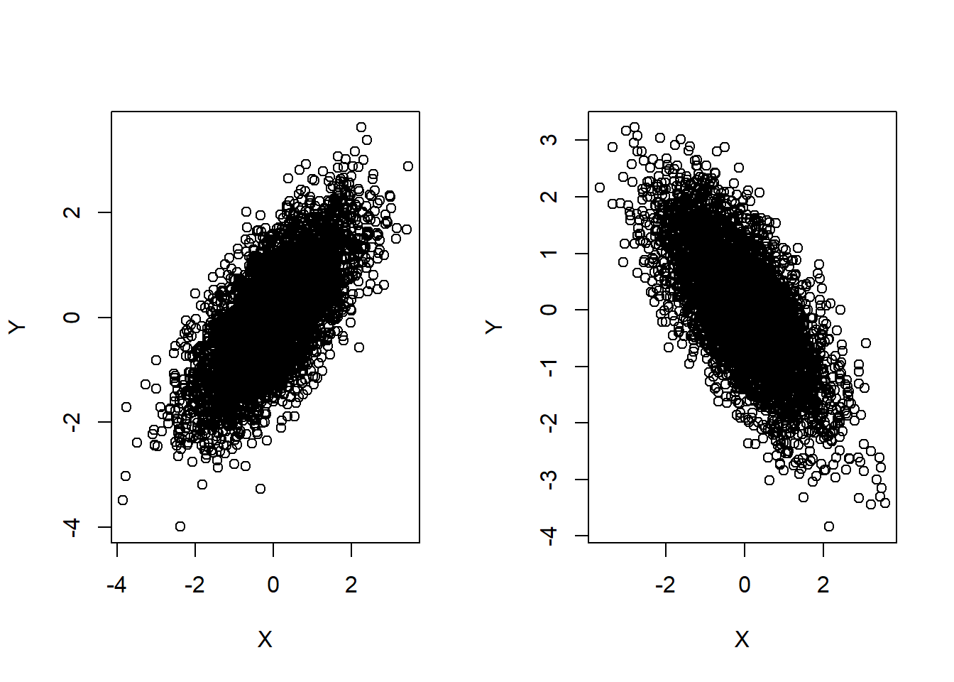
Figure 5.1: Positive Covariance (Left), Negative Covariance (Right)

One more thing to note: covariance and correlations can be calculated for random variables as long as they are quantitative, but not if at least one of them is categorical. The concept of increasing a random variable that is categorical does not make intuitive sense, for example, if we have a random variable that denotes the color of eyes, what does increasing color of eyes mean?

5.4.1 Covariance

We now define covariance. The covariance between random variables \(X\) and \(Y\) is

\[\begin{equation} Cov(X,Y) = E\left[(X- \mu_X)(Y - \mu_Y) \right]. \tag{5.20} \end{equation}\]

Looking at equation (5.20), we see that if both \(X\) and \(Y\) generally move in the same direction, then \(X - \mu_x\) and \(Y - \mu_y\) will either be both positive or both negative, therefore their product is positive, on average. If \(X\) and \(Y\) generally move in opposite directions, then \(X - \mu_x\) and \(Y - \mu_y\) have opposite signs, therefore their product is negative, on average.

Some key properties for covariance:

• \(Cov(X,X) = Var(X)\).The covariance of any random variable with itself is its variance.
• \(Cov(X,Y) = Cov(Y,X)\). The covariance between \(X\) and \(Y\) is the same as the covariance between \(Y\) and \(X\).
• \(Cov(X,c) = 0\) for any constant \(c\). Since a constant does not move, it has no relationship with \(X\).
• \(Cov(aX,Y) = a Cov(X,Y)\) for any constant \(a\). This implies that covariance is affected by the units of \(X\) and \(Y\).
• \(Var(X + Y) = Var(X) + Var(Y) + 2 Cov(X,Y)\).
• If \(X\) and \(Y\) are independent, then \(Cov(X,Y) = 0\).
• However, \(Cov(X,Y) = 0\) does not mean that \(X\) and \(Y\) are independent. This is a common misconception. Remember that covariance measures linear relationship. The relationship between \(X\) and \(Y\) could be non linear, and in such instances, the covariance should not be used. Figure 5.2 below provides an example this. In this figure, \(X\) and \(Y\) have a quadratic relationship, so they are clearly not independent, yet their covariance is virtually 0.

x<-seq(-1,1, by=0.01)
y<-x^2

##note from plot that X & Y do not have a linear relationship
plot(x,y, xlab="X", ylab="Y")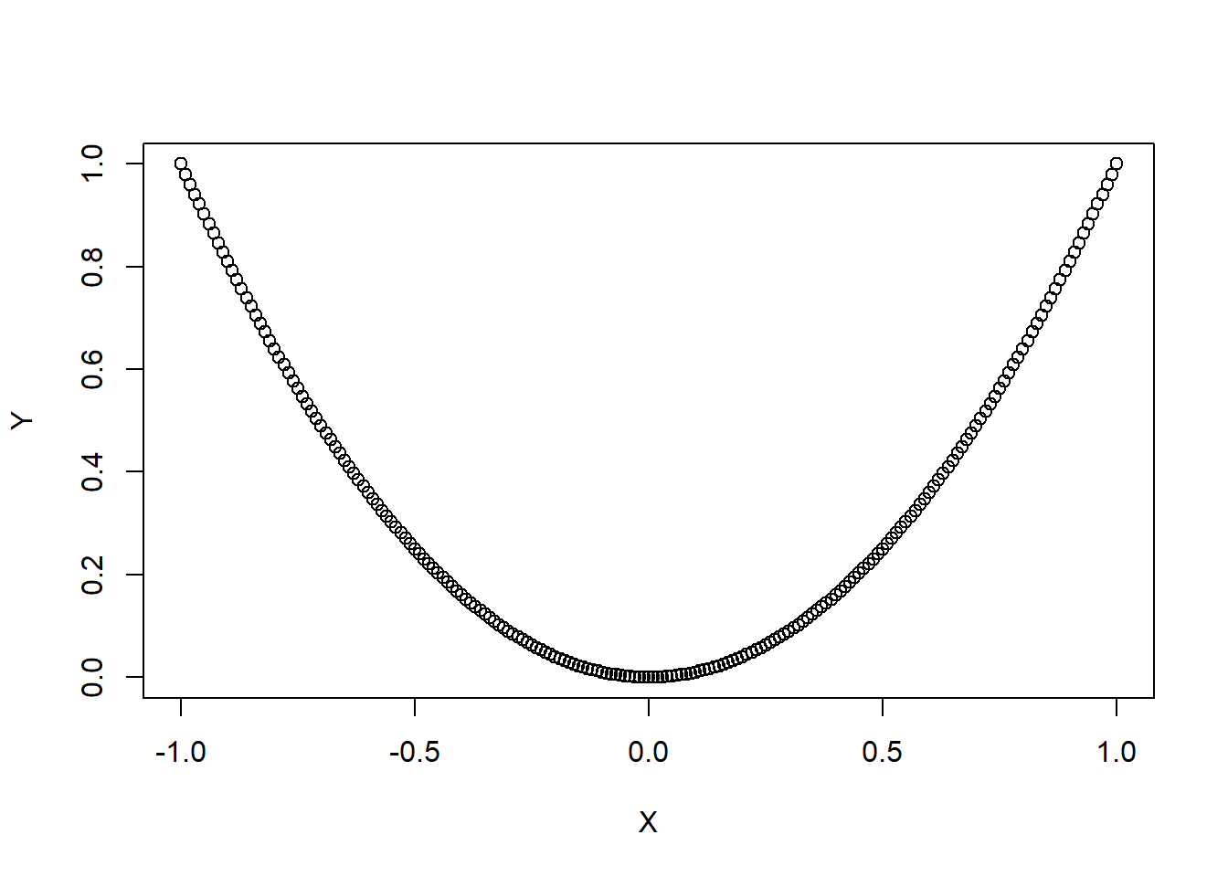

Figure 5.2: Covariance with Non Linear Relationship

cov(x,y) ##covariance is virtually 0

## [1] 1.19967e-17

Suppose we have two vectors of observed data, each of size \(n\): \(X = (x_1, x_2, \cdots, x_n)\) and \(Y = (y_1, y_2, \cdots, y_n)\). Their sample covariance is

\[\begin{equation} s_{x,y} = \frac{\sum_{i=1}^n (x_i - \bar{x})(y_i - \bar{y})}{n-1} \tag{5.21} \end{equation}\]

We noted earlier that covariance is affected by the units of the variables. Suppose one variable is measured in meters, and we convert it to become centimeters. The value of the covariance will get multiplied by 100. People find it easier to interpret a measure that does not depend on the units. This is where the correlation comes in: it is a unitless version of the covariance.

View the video below for a visual explanation as to why the sample covariance is positive when the linear relationship is positive:

5.4.2 Correlation

The correlation between random variables \(X\) and \(Y\) is

\[\begin{equation} \rho = Corr(X,Y) = \frac{Cov(X,Y)}{\sqrt{Var(X) Var(Y)}}. \tag{5.22} \end{equation}\]

The sample correlation for two vectors of observed data, each of size \(n\): \(X = (x_1, x_2, \cdots, x_n)\) and \(Y = (y_1, y_2, \cdots, y_n)\), is

\[\begin{equation} r = \frac{\sum_{i=1}^n (x_i - \bar{x})(y_i - \bar{y})}{\sqrt{\sum_{i=1}^n (x_i - \bar{x})^2 \sum_{i=1}^n (y_i - \bar{y})^2}} \tag{5.23} \end{equation}\]

Some key properties of correlation:

• It is bounded between -1 and 1.
• Values closer to -1 or 1 indicate a stronger linear relationship.
• Values closer to 0 indicate a weaker linear relationship.
• Its numerical value is unchanged with location and / or scale changes.
• If \(X\) and \(Y\) are independent, then \(Corr(X,Y) = 0\).
• However, \(Corr(X,Y) = 0\) does not mean that \(X\) and \(Y\) are independent.
• Correlation should only be used if the relationship between \(X\) and \(Y\) is linear.

Figure 5.3 below shows examples of some scatterplots and their sample correlations. For the left plot, the data points fall close to a straight line, is negative, and so its correlation is close to -1. The middle plot has no linear relationship, so we do not see a trend with one variable increasing or decreasing as the other variable increases. The right plot shows the data points being fairly close to a straight line, but not as close as the left plot), so its correlation is not as close to 1 (or -1).

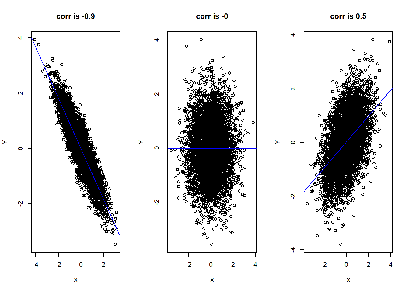
Figure 5.3: Strong Negative Correlation (Left), No Correlation (Middle), Moderate Positive Correlation (Right)

5.5 Conditional Expectation

In Section 2.3 and 5.2.2, we explored the notion of conditional probabilities and conditional distributions, which are used for:

• Updating the probability and distribution of a random variable \(Y\), after observing a certain outcome of another random variable \(X\), or
• Restricting the probability and distribution of a random variable \(Y\) to a certain value of another random variable.

These represent the Bayesian and frequentist viewpoints of conditional probability and conditional distribution.

It turns out a similar idea applies to the expected value of a random variable. Recall that the expected value of a random variable is the long-run average, in other words, the average value after observing the random variable an infinite number of times.

The conditional expectation of a random variable is its long run-average:

• after observing a certain outcome of another variable or event, or
• after restricting our attention to cases when another random variable is fixed or equal to a specific value.

Fairly often, we use statistical models to predict a response variable \(Y\) based on a predictor \(X\). Predictions for values of \(Y\) based on observed values of \(X\) usually use the conditional expectation of \(Y\) given \(X\). Given what we see with the predictor, the long run average of \(Y\) ends up being used as the predicted value of the response variable. This is the basis for most statistical models.

There are two slightly different notions of conditional expectations:

• Conditional expectation of random variable \(Y\) given event \(A\). If \(A\) has happened, what is the expected value of \(Y\)?
• Conditional expectation of random variable \(Y\) given another random variable \(X\). If we fix the value of the random variable \(X\) to any value on its support, what is the expected value of \(Y\)?

The second notion is the one that is usually used for statistical models, but we will cover both as the first notion is easier to understand, and should help us understand the second notion.

5.5.1 Conditional Expectation Given Event

Recall that the expectation \(E(Y)\) of a random variable \(Y\) is its long-run average. If \(Y\) is discrete, we take a weighted average involving the probabilities in its PMF \(P(Y=y)\). The calculation of the conditional expectation \(E(Y|A)\) where \(A\) is an event that has occurred simply replaces the probabilities \(P(Y=y)\) with conditional probabilities \(P(Y=y|A)\). Therefore, for a discrete random variable \(Y\),

\[\begin{equation} E(Y|A) = \sum_y y P(Y=y|A) \tag{5.24} \end{equation}\]

where the sum is over the support of \(Y\). Notice how we are summing the product of the support with its corresponding conditional probability, whereas to find \(E(Y)\), we sum the product of the support with its corresponding unconditional probability.

If \(Y\) is continuous, we use the conditional PDF instead:

\[\begin{equation} E(Y|A) = \int_{-\infty}^{\infty} y f(y|A) dy. \tag{5.25} \end{equation}\]

The key is to understand the intuition behind conditional expectations, and we will use simulation to approximate this (the approximation works better if we use more simulated data). Simulation represents the frequentist viewpoint of conditional expectation. The code below does the following:

• Generate 100 values of \(X\) uniformly on the support \(\{1,2,3,4\}\).
• Simulate \(Y\) using \(Y = 10 + X + \epsilon\) where \(\epsilon \sim N(0,1)\).
• Represent these values on a scatter plot, and also overlay a line that represents the sample mean of \(Y\), which estimates \(E(Y)\). This is simply the average value on the y-axis for all 100 data points. This is the plot on the left in Figure 5.4 below.
• Represent these values on a scatter plot, but use blue to denote the event \(A\) which is when \(X=1\). A line that represents the sample mean of \(Y\), only for these blue data points (i.e. only when \(X=1\)), is overlaid. This value estimates \(E(Y|A)\) or \(E(Y|X=1)\). This is the plot on the right in Figure 5.4 below. In calculating this sample mean, we could have completed disregarded the black data points when \(X\) was not 1.

set.seed(40)
n<-100 ##100 data points

##generate X
x<-c(rep(1,n/4), rep(2,n/4), rep(3,n/4), rep(4,n/4)) 

##simulate Y
y<- 10 + x + rnorm(n)

par(mfrow=c(1,2))
plot(x,y, main="Estimated E(Y) Overlaid")
abline(h=mean(y)) ##add line to represent est E(Y)

plot(x,y, col = ifelse(x == 1,'blue', 'black'), pch = 19, main="Estimated E(Y|X=1) Overlaid" )
abline(h=mean(y[x=1]), col="blue") ##add line to represent est E(Y|X=1)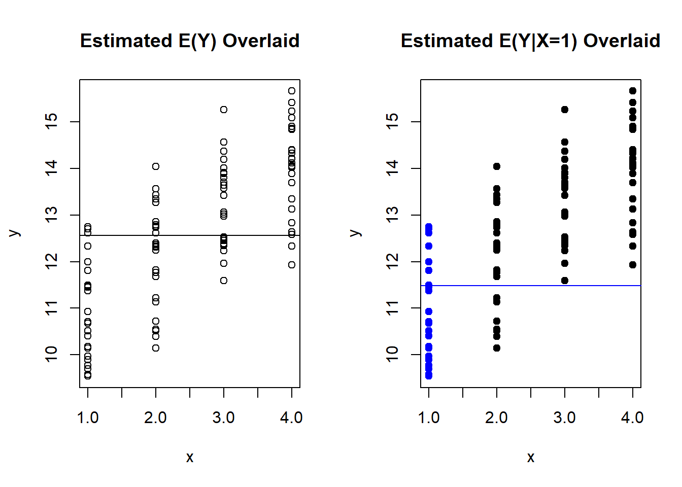

Figure 5.4: Comparison of E(Y) and E(Y|X=1)

So, we can interpret the conditional expectation \(E(Y|A)\) as the long-run average of \(Y\) (only) when \(A\) has happened. It is the long-run average of \(Y\) when a certain condition is met.

View the video below for a more detailed explanation for this simulation:

5.5.2 Conditional Expectation Given Random Variable

The conditional expectation of \(Y\) given a random variable \(X\) is slightly different. In the simulated example in the previous subsection, we set \(X\) to be a specific value. Now, we consider the long-run average of \(Y\) for each value, instead of a specific value, in the support of \(X\).

One way to think about this is to consider \(E(Y|X=x)\), where \(x\) is any value on the support for \(X\). If \(Y\) is discrete, this conditional expectation is:

\[\begin{equation} E(Y|A) = \sum_y y P(Y=y|X=x) \tag{5.26} \end{equation}\]

where the sum is over the support of \(Y\).

If \(Y\) is continuous:

\[\begin{equation} E(Y|A) = \int_{-\infty}^{\infty} y f(y|x) dy. \tag{5.27} \end{equation}\]

We go back to the simulated example in the previous subsection to explain what \(E(Y|X=x)\) represents. Recall that the support for \(X\) is \(\{1,2,3,4\}\) and that \(Y = 10 + X + \epsilon\) where \(\epsilon \sim N(0,1)\). So

\[ \begin{split} E(Y|X=x) &= E(10 + X + \epsilon | X=x)\\ &= E(10 + x + \epsilon) \\ &= E(10) + E(x) + E(\epsilon) \\ &= 10 + x + 0 \\ &= 10 + x. \end{split} \]

A brief explanation of each step:

• To go from line 1 to line 2, we subbed in \(x\) for \(X\), since we are setting \(X=x\).
• To go from line 2 to line 3, we apply the linearity of expectations.
• To go from line 3 to 4, \(E(c)=c\) for any constant. In this case, we are fixing \(x\) to be a value in the support so it is a constant, and \(E(\epsilon) = 0\) since \(\epsilon \sim N(0,1)\).

So \(E(Y|X) = 10 + X\). What this means is that:

• When \(X=1\), \(E(Y|X=1) = 11\),
• When \(X=2\), \(E(Y|X=1) = 12\),
• When \(X=3\), \(E(Y|X=1) = 13\), and
• When \(X=4\), \(E(Y|X=1) = 14\).

Note: We set up \(Y = 10 + X + \epsilon\) where \(\epsilon \sim N(0,1)\) in the simulation. This follows the framework for linear regression which sets up \(Y = \beta_0 + \beta_1 X + \epsilon\) where \(\epsilon \sim N(0,\sigma^2)\), i.e. \(\epsilon\) is normal with mean 0 and a variance that is a fixed value. The conditional expectation given \(X\) ends up being the prediction for \(Y\) that minimizes the mean squared error in linear regression.

View the video below for a more detailed explanation of this example:

5.6 Common Multivariate Distributions

We now cover two of the most common multivariate distributions: the multinomial distribution and multivariate normal distribution for discrete and continuous random variables respectively.

5.6.1 Multinomial

The multinomial distribution can be viewed as a generalization of the binomial distribution into higher dimensions. Recall that for the binomial distribution, we carry out \(n\) trials, and for each trial we record whether it as a success or failure, in other words, there are only two outcomes for each trial. The multinomial distribution differs in that there can be more than two outcomes for each trial. For example, we randomly select \(n\) adults and ask them for their political affiliation. The affiliation could be Democrat, Republican, other party, or no affiliation, so there are four possible outcomes or categories for each person.

The set up of the multinomial distribution is as follows:

• We have \(n\) independent trials, and each trial belongs to one of \(k\) categories.
• Each trial belongs to category \(j\) with probability \(p_j\), where \(p_j\) is non negative and \(\sum_{j=1}^k p_j = 1\), i.e. they sum to one.
• Let \(X_1\) denote the number of trials belonging to category 1, \(X_2\) denote the number of trials belonging to category 2, and so on. Then \(X_1 + \cdots X_k = n\).

We then say that \(\boldsymbol{X} = (X_1, \cdots, X_k)\) is said to have a multinomial distribution with parameters \(n\) and \(\boldsymbol{p} = (p_1, \cdots, p_k)\). This can be written as \(\boldsymbol{X} \sim Mult_k(n, \boldsymbol{p})\).

Note that the vectors \(\boldsymbol{X}\) and \(\boldsymbol{p}\) are written in bold. Vectors and matrices are commonly written using bold to distinguish them from scalars, which are not in bold. \(\boldsymbol{X}\) is an example of what we call a random vector, as it is a vector of random variables \(X_1, \cdots, X_k\).

If \(\boldsymbol{X} \sim Mult_k(n, \boldsymbol{p})\), its PMF is

\[\begin{equation} P(X_1 = n_1, \cdots, X_k = n_k) = \frac{n!}{n_{1}! \cdots n_{k}!} p_1^{n_1} \cdots p_k^{n_k}, \tag{5.28} \end{equation}\]

where \(n_1 + \cdots + n_k = n\).

Let us use a toy example. Going back to political affiliations. Suppose among American voters, 28% identify as Democrats, 29% identify as Republicans, and 10% identify have other affiliations, and 33% are independents. Let \(X_1, X_2, X_3, X_4\) denote the number of Democrats, Republicans, others, and independents. The joint distribution of \(X_1, X_2, X_3, X_4\) is \(\boldsymbol{X} = (X_1, X_2, X_3, X_4) \sim Mult_4(0.28, 0.29, 0.1, 0.33)\).

Suppose we want to find the probability that in a sample of 10 voters, 2 are Democrats, 3 are Republicans, and 1 has another affiliation, and 4 are Independents:

\[ \begin{split} P(X_1 = 2, X_2 = 3, X_3 = 1, X_4 = 4) &= \frac{10!}{2! 3! 1!4!} 0.28^{2} 0.29^{3} 0.1^1 0.33^4\\ &= 0.02857172. \end{split} \]

Or use

dmultinom(c(2,3,1,4), prob=c(0.28,0.29,0.1,0.33)) ##specify X1, X2, X3, X4, then p1,p2,p3, p4

## [1] 0.02857172

5.6.1.1 Multinomial Marginals

The marginals of a multinomial are binomial. For \(\boldsymbol{X} \sim Mult_k(n, \boldsymbol{p})\), \(X_j \sim Bin(n, p_j)\).

Going back to our toy example with American voters, this means that \(X_1 \sim Bin(n,0.28), X_2 \sim Bin(n,0.29), X_3 \sim Bin(n, 0.1), X_4 \sim Bin(n,0.33)\). Hopefully this example makes sense. If we look at \(X_1,\) we are looking at the number of voters who are democrats and those who are not. The proportion of Democrats still remains the same, while the proportion of Republicans, other affiliations, and independents is the sum of their individual proportions, or 1 minus the proportion of Democrats.

5.6.1.2 Multinomial Lumping

With discrete and categorical variables, it can be common to want to lump (or merge, or collapse, or combine) categories together. If \(\boldsymbol{X} \sim Mult_k(n, \boldsymbol{p})\), then \(X_i + X_j \sim Bin(n, p_i + p_j)\). If we decide to merge categories 1 and 2, we have \((X_1 + X_2, X_3, \cdots, X_k) \sim Mult_{k-1}(n, (p_1 + p_2, p_3, \cdots, p_k))\).

We go back to our toy example. Suppose we consider Democrats and Republicans to be the major parties, we may wish to combine everyone else into one category: those with other affiliations and independents. We can define this using a new random variable \(\boldsymbol{Y} = (X_1, X_2, X_3+X_4) \sim Mult_3(n,(0.29,0.29,0.43)\). Note we now have 3 categories instead of 4. The proportion for the lumped category is the sum of their individual proportions.

5.6.1.3 Multinomial Covariance

For \(\boldsymbol{X} \sim Mult_k(n, \boldsymbol{p})\) with \(\boldsymbol{p} = (p_1,p_2, \cdots, p_k)\). The covariance between any two distinct components \(X_i\) and \(X_j\) is

\[\begin{equation} Cov(X_i, X_j) = -n p_i p_j, \tag{5.29} \end{equation}\]

for any \(i \neq j\). The book provides a nice proof, under Theorem 7.4.6, for those interested.

Looking at (5.29), we notice the covariance between any two distinct components is negative (since probabilities are non negative). This means that the numerical values of \(X_i\) and \(X_j\) go in opposite directions. This should make intuitive sense since \(n = X_1 + \cdots + X_k\) is fixed, so if \(X_i\) is large, \(X_j\) should be small since \(n\) is fixed. An extreme example will be if \(X_i = n\), then \(X_j\) must be 0.

We go back to our toy example. Suppose we want to find the correlation between \(X_1\) and \(X_2\), the number of Democrats and Republicans in a sample of size \(n\). Note that \(X_1 \sim Bin(n,0.28), X_2 \sim Bin(n,0.29)\), and \(Cov(X_1,X_2) = -n \times 0.28 \times 0.29 = 0.0812n\),

\[ \begin{split} Corr(X_1,X_2) &= \frac{Cov(X_1,X_2)}{\sqrt{Var(X_1) Var(X_2)}}\\ &= \frac{-n p_1 p_2}{\sqrt{n p_1 (1-p_1) n p_2 (1-p_2)}} \\ &= -\sqrt{\frac{p_1 p_2}{(1-p_1)(1-p_2)}} \\ &= -\sqrt{\frac{0.28 \times 0.29}{(1-0.28)(1-0.29)}} \\ &= -0.3985498. \end{split} \]

5.6.1.4 Conditional Multinomial

Sometimes, we have some observed data from a multinomial distribution, and wish to update the distribution. Suppose we have \(\boldsymbol{X} \sim Mult_k(n, \boldsymbol{p})\), and we observed that \(X_1 = n_1\), then \((X_2, \cdots, X_k)|X_1 = n_1 \sim Mult_{k-1}(n-n_1, (p_2^{\prime}, \cdots, p_k^{\prime}))\) where \(p_j^{\prime} = \frac{p_j}{p_2 + \cdots + p_k}\).

5.6.2 Multivariate Normal

The multivariate normal (MVN) distribution can be viewed as a generalization of the normal distribution into higher dimensions. Just like the univariate normal distribution, the central limit theorem also applies to higher dimensions.

A \(k\)-dimensional random vector \(\boldsymbol{X} = (X_1, \cdots, X_k)\) is said to have an MVN distribution if every linear combination of the \(X_j\) is normal. This means that \(t_1 X_1 + \cdots + t_k X_k\) is normally distributed for any constants \(t_1, \cdots, t_k\). When \(k=2\), the MVN is often called a bivariate normal.

In Section 4.5.2.2, we mentioned that the parameters of a normal distribution are its mean \(\mu\) and variance \(\sigma^2\). This idea is generalized to a MVN \(\boldsymbol{X} = (X_1, \cdots, X_k)\). The parameters are:

• the mean vector \((\mu_1, \cdots, \mu_k)\) where \(\mu_j = E(X_j)\). This is a vector of length \(k\) where each entry is the expected value of that component.

• the covariance matrix. This is a \(k \times k\) matrix where the \((i,j)\)th entry (i.e. row \(i\), column \(j\)) is the covariance between \(X_i\) and \(X_j\). This implies that the diagonal entries give the variance of each component (since \(Cov(X_i, X_i) = Var(X_i)\)), and the covariance matrix is symmetric (since \(Cov(X_i, X_j) = Cov(X_j, X_i)\)).

For example, suppose we have \(\boldsymbol{X} = (X_1, X_2, X_3)\) that is MVN with mean vector \((5, 2, 8)\) and covariance matrix

\[ \begin{pmatrix} 3 & 1.5 & 2.5\\ 1.5 & 2 & 4.2 \\ 2.5 & 4.2 & 1 \end{pmatrix}, \]

then

• \(E(X_1) = 5, E(X_2) = 2, E(X_3) = 8\),
• \(Var(X_1) = 3, Var(X_2) = 2, Var(X_3) = 1\),
• \(Cov(X_1, X_2) = Cov(X_2, X_1) = 1.5\),
• \(Cov(X_1, X_3) = Cov(X_3, X_1) = 2.5\), and
• \(Cov(X_2, X_3) = Cov(X_3, X_2) = 4.2\).

Some properties of the MVN distribution:

1. If \(\boldsymbol{X} = (X_1, \cdots, X_k)\) is MVN, the marginal distribution of each \(X_j\) is normal, as we can set \(t_j =1\) and all other constants to be 0.

2. However, the converse is not necessarily true. If each \(X_1, \cdots, X_k\) is normal, \((X_1, \cdots, X_k)\) is not necessarily MVN.

3. If \((X_1, \cdots, X_k)\) is MVN, then so is any subvector, e.g. \((X_i, X_j)\) is bivariate normal.

4. If \(\boldsymbol{X} = (X_1, \cdots, X_k)\) and \(\boldsymbol{Y} = (Y_1, \cdots, Y_m)\) are MVN with \(\boldsymbol{X}\) independent of \(\boldsymbol{Y}\), then \(\boldsymbol{W} = (X_1, \cdots, X_k, Y_1, \cdots, Y_m)\) is MVN.

5. Within an MVN random vector, uncorrelated implies independence. If \(\boldsymbol{X}\) is MVN and \(\boldsymbol{X} = (\boldsymbol{X_1, X_2})\) where \(\boldsymbol{X_1}\) and \(\boldsymbol{X_2}\) are subvectors, and every component of \(\boldsymbol{X_1}\) is uncorrelated with every component of \(\boldsymbol{X_2}\), then \(\boldsymbol{X_1}\) and \(\boldsymbol{X_2}\) are independent.

5.6.2.1 Simulations

We can use simulations to verify the first property. For this simulation, we will do the following:

• Simulate 5000 draws from a MVN distribution with mean vector \((1,2,5)\) and covariance matrix

\[ \begin{pmatrix} 1 & 0.5 & 0.6\\ 0.5 & 2 & 0.2 \\ 0.6 & 0.2 & 4 \end{pmatrix}. \]

• Assess if each component \(X_1, X_2, X_3\) is normally distributed by using the Shapiro-Wilk test for normality.

  • The null hypothesis is that the variable follows a normal distribution, and the alternative hypothesis is that the variable does not follow a normal distribution.
  • So rejecting the null hypothesis means the variable is inconsistent with a normal distribution, while not rejecting means we do not have evidence the variable is inconsistent with a normal distribution.
  • We will record the p-value of each test on \(X_1, X_2, X_3\).

• Repeat the previous 2 steps for a total of 10 thousand reps.

• Count the proportion of reps where the Shapiro-Wilk test rejected the null hypothesis at significance level 0.05 for \(X_1, X_2, X_3\).

  • If this property is correct, we will expect close to 5% of the p-values to (wrongly) reject the null hypothesis, since the tests are conducted at 0.05 significance level.

library(mvtnorm) ##package to simulate from MVN

reps<-1000 ## how many reps
pvalsx1<-pvalsx2<-pvalsx3<-array(0,reps) ##initialize an array to store the pvalues from each test at each rep
siglevel<-0.05 ##sig level
n<-5000 ##number of draws for each rep

mu_vector<-c(1,2,5) ##mean vector

##set up covariance matrix
sig12<-0.5
sig13<-0.6
sig23<-0.2
cov_mat<-matrix(c(1,sig12,sig13,sig12,2,sig23,sig13,sig23,4), nrow=3, ncol=3)

##set.seed so you can replicate my result.
set.seed(30)

##run steps 1 and 2 for 10 000 times
for (i in 1:reps)
  
{

  data<-rmvnorm(n, mu_vector, cov_mat)
  
  x1<-data[,1] ##extract X1
  x2<-data[,2] ##extract X2
  x3<-data[,3] ##extract X3
  
  ##store pvalue from Shapiro-Wilk test from each component
  pvalsx1[i]<-shapiro.test(x1)$p.value 
  pvalsx2[i]<-shapiro.test(x2)$p.value
  pvalsx3[i]<-shapiro.test(x3)$p.value 
  
}

##proportion of tests that wrongly reject the null
sum(pvalsx1<siglevel)/reps ##for X1

## [1] 0.054

sum(pvalsx2<siglevel)/reps ##for X2

## [1] 0.037

sum(pvalsx3<siglevel)/reps ##for X3

## [1] 0.047

Since close to 5% of each hypothesis test rejected the null hypothesis, it appears that each component is consistent with a normal distribution. (Or more accurately, we do not have evidence to say that each component is not normal.) It does appear that if \(\boldsymbol{X} = (X_1, \cdots, X_k)\) is MVN, the marginal distribution of each \(X_j\) is normal. Our simulation does not provide evidence against this property.

Note: What we have done is called a Monte Carlo simulation, and is often used in research to verify theorems. While you may not be involved in research, writing code to run simulations is a good way for you to understand these theorems and how they are applied. We will cover Monte Carlo simulations in more detail in a later module.