7 Estimation

This module is based on Introduction to Probability for Data Science (Chan), Chapter 8.1 and 8.2. You can access the book for free at https://probability4datascience.com. Please note that I cover additional topics, and skip certain topics from the book. You may skip Section 8.1.3, 8.1.4, and 8.1.6 from the book.

7.1 Introduction

We consider building models based on the data we have. Many models are based on some distribution, for example, the linear regression model is based on the normal distribution, and the logistic regression model is based on the Bernoulli distribution. Recall that these distributions are specified by their parameters: the mean \(\mu\) and variance \(\sigma^2\) for the normal distribution, and the success probability \(p\) for a Bernoulli distribution. The value of the parameters are almost always unknown in real life. This module deals with estimation: how we estimate the values of these parameters, as well as quantify the level of uncertainty we have with these estimated values, given the data we have.

7.1.1 Big Picture Idea with Estimation

Consider this simple scenario. We want to find the distribution associated with the systolic blood pressure of American adults. To be able to achieve this goal, we would have to get the systolic blood pressure of every single American adult. This is usually not feasible as researchers are unlikely to have the time and money to interview every single American adult. Instead, a representative sample of American adults will be obtained, for example, 750 randomly selected American adults are interviewed. We can then create density plots, histograms, compute the mean, median, variance, skewness, and other summaries that may be of interest, based on these 750 American adults.

7.1.1.1 Population Vs Sample

The above scenario illustrates a few concepts and terms that are fundamental in estimation. In any study, we must be clear as to who or what is the population of interest, and who or what is the sample.

The population (sometimes called the population of interest) is the entire set of individuals, or objects, or events that a study is interested in. In the scenario described above, the population would be (all) American adults.

The sample is the set of individuals, or objects, or events which we have data on. In the scenario described above, the sample is the 750 randomly selected American adults.

Ideally, the sample should be representative of the population. A representative sample is often achieved through a simple random sample, where each unit in the population has the same chance of being selected to be in the sample. In this module, we will assume that we have a representative sample. Note: You may feel that obtaining a simple random sample may be difficult. We will not get into a discussion of sampling (sometimes called survey sampling), which is a field of statistics that handles how to obtain representative samples, or how calculations should be adjusted if the sample is not representative. There is still a lot of research that is being done in survey sampling.

7.1.1.2 Variables & Observations

A variable is a characteristic or attribute of individuals, or objects, or events that make up the population and sample. In the above scenario, a variable would be the systolic blood pressure of American adults. We can use the notation of random variables to describe variables. For example, we can let \(X\) denote the systolic blood pressure of an American adult, so writing \(P(X>200)\) means we want to find the probability that an American adult has systolic blood pressure greater than 200 mm Hg .

An observation is the individual person, object or event that we collect data from. In the above scenario, an observation is a single American adult in our sample of 750.

One way to think about variables and observations is through a spreadsheet. Typically, each row represents an observation and each column represents a variable. Figure 7.1 below displays such an example, based on the described scenario. Each row represents an observation, i.e. a single American adult in our sample, and the column represents the variable, which is systolic blood pressure.

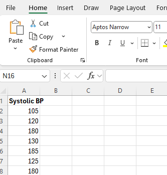
Figure 7.1: Example of Data in a Spreadsheet

7.1.1.3 Parameter Vs Estimator

Now that we have made the distinction between a population and a sample, we are ready to define parameters and estimators.

A parameter is a numerical summary associated with a population. In the scenario described above, an example of a population parameter would be the population mean systolic blood pressure of American adults.

An estimator is a numerical summary associated with samples. An estimator is typically used to estimate a parameter. In the scenario described above, an estimator of the population mean systolic blood pressure of American adults could be the average systolic blood pressure in our sample. So the sample mean is an estimator of the population mean.

An estimated value, or estimate, is the actual value of the estimator based on a sample. In the scenario described above, suppose the average systolic blood pressure of the 750 American adults is 140 mm Hg. We will say the estimated value of the mean systolic blood pressure of American adults is 140 mm Hg.

So a parameter is a number that is associated with a population, while an estimator is a number that is associated with a sample. Some other differences between parameters and estimators:

• The value of parameters are unknown, while we can actually calculate numerical values of estimators.
• The value of parameters are considered fixed (as there is only one population), while the numerical values of estimators can vary if we obtain multiple random samples of the same sample size. Using the scenario above again, suppose we obtain a second representative sample of 750 American adults. The average systolic blood pressure of this second sample is likely to be different from the average systolic blood pressure of the first sample. This illustrates that there is variance, or uncertainty, associated with estimators due to random sampling. This is the uncertainty that we will be focusing on in this section.

Whenever we propose an estimator for a parameter, we want to assess how “good” the estimator is. In some situations, there is an obvious choice for an estimator, for example, using the sample mean, \(\bar{x} = \frac{\sum x_i}{n}\) to estimate the population mean. But in some instances, the choice may not be so obvious. For example, why do use the sample variance \(s^2 = \frac{\sum (x_i - \bar{x})^2}{n-1}\) as an estimator for the population variance, and not \(\frac{\sum (x_i - \bar{x})^2}{n}\)? We will cover a few measures that are used to assess an estimator: bias, variance, and mean-squared error.

We will also cover a couple of methods in estimating parameters: the method of moments, and the method of maximum likelihood. You will notice that we use probability rules in these methods.

To sum up estimation: we use data from a sample to estimate unknown characteristics of a population, so that we can answer questions regarding variables in the population, as well as provide a measure of uncertainty for our answers.

7.1.2 Module Roadmap

• Section 7.2 covers estimation using the method of moments. This method is fairly intuitive, although it is not as commonly used as it lacks certain ideal properties.
• Section 7.3 covers estimation using the method of maximum likelihood. This method is a workhorse in statistics and probability as many models are estimated using this method.
• Section 7.4 covers measures that are used to evaluate how “good” an estimator is.
• Section 7.5 provides some final comments on estimation.

7.2 Method of Moments Estimation

We will cover a couple of methods in estimation. The first method is the method of moments. It is a more intuitive method, although it lacks certain ideal properties. Before defining this method, we recall and define some terms.

In Section 4.4.3, we defined moments. As a reminder, for a random variable \(X\), its \(k\)th moment is \(E(X^k)\), which can be found using LOTUS: \(\int_{-\infty}^{\infty} x^k f_X(x) dx\).

Suppose we observe a random sample \(x_1, \cdots, x_n\) that comes from \(X\). The \(k\)th sample moment is \(M_k = \frac{1}{n} \sum_{i=1}^n x_i^k\).

Using these definitions,

• The 1st moment is \(E(X) = \mu_x\), the population mean of \(X\).
• The 1st sample moment is \(M_1 = \frac{1}{n} \sum_{i=1}^n x_i = \bar{x}\), the sample mean.
• The 2nd moment is \(E(X^2)\).
• The 2nd sample moment is \(M_2 = \frac{1}{n} \sum_{i=1}^n x_i^2\).

And so on.

The method of moments estimation is: Let \(X\) be a random variable with distribution depending on parameters \(\theta_1, \cdots, \theta_m\). The method of moments (MOM) estimates \(\hat{\theta}_1, \cdots, \hat{\theta}_m\) are found by equating the first \(m\) sample moments to the corresponding first \(m\) moments and solving for \(\theta_1, \cdots, \theta_m\).

You might have noticed that the method of moments is based on the Law of Large Numbers.

Note: By convention, parameters are typically denoted by Greek letters, and their estimators are denoted with a hat symbol over the corresponding letter.

Let us look at a couple of examples:

1. Suppose I have a coin and I do not know if it is fair or not. There are only two outcomes on a flip, heads or tails. Each flip is independent of other flips. Let \(X_i\) denote whether the \(i\)th flip lands heads, where \(X_i = 1\) if heads and \(X_i = 0\) if tails. We can see that \(X_i \sim Bern(p)\), where \(p\) is the probability it lands heads. Derive the MOM estimate for \(p\).

A Bernoulli distribution has only 1 parameter, \(p\), so when using the method of moments, we only need to equate the first sample moment to the first moment.

• The first moment is \(E(X_i) = p\), since \(X_i \sim Bern(p)\).
• The first sample moment is \(M_1 = \frac{1}{n} \sum_{i=1}^n x_i = \bar{x}\).

Set \(E(X_i) = M_1\), i.e. \(\hat{p} = \bar{x}\). Since \(X_i = 1\) if heads and \(X_i = 0\) if tails, \(\frac{1}{n} \sum_{i=1}^n x_i = \bar{x}\) actually represents the proportion of flips that land on heads, based on \(n\) flips. So this is actually the sample proportion.

The MOM estimate for this problem is \(\hat{p}\), the proportion of \(n\) flips that land on heads. This result should be fairly intuitive. If we flip a coin a large number of times, and 70% of the flips land on heads, the sample proportion is \(\hat{p} = 0.7\), and so the estimated value for \(p\), the success probability is 0.7.

2. Birth weights of newborn babies typically follow a normal distribution. We have data from births at Baystate Medical Center in Springfield, MA, during 1986. Assuming that the births at this hospital is representative of births in New England in 1986, derive the MOM estimates for \(\mu\) and \(\sigma^2\), the mean and variance of the distribution of birth weights in New England in 1986.

A normal distribution has 2 parameters, \(\mu\) and \(\sigma^2\), so we need to equate the first two sample moments to the first two moments. Let \(X\) denote the birth weights in New England in 1986, so \(X \sim N(\mu, \sigma^2)\).

• The first moment is \(E(X) = \mu\), since \(X \sim N(\mu, \sigma^2)\).
• The first sample moment is \(M_1 = \frac{1}{n} \sum_{i=1}^n x_i = \bar{x}\).

So we set \(E(X) = M_1\), i.e. \(\hat{\mu} = \bar{x}\). This is just the sample average of the birth weights at Baystate Medical Center in 1986.

• The second moment is \(E(X^2)\). But we know that since \(X \sim N(\mu, \sigma^2)\).

\[ \begin{split} Var(X) &= E(X^2) - E(X)^2\\ \implies E(X^2) &= Var(X) + E(X)^2 \\ \implies E(X^2) &= \sigma^2 + \mu^2 \end{split} \]

• The second sample moment is \(M_2 = \frac{1}{n} \sum_{i=1}^n x_i^2\).

So we set \(E(X^2) = M_2\), i.e. \(\hat{\sigma^2} + \hat{\mu}^2 = \frac{1}{n} \sum_{i=1}^n x_i^2\). Since we earlier found that \(\hat{\mu} = \bar{x}\), we get \(\hat{\sigma^2} = \frac{1}{n} \sum_{i=1}^n x_i^2 - \bar{x}^2 = \frac{1}{n} \sum_{i=1}^n (x_i - \bar{x})^2\).

Therefore, the MOM estimates for \(\mu\) and \(\sigma^2\) are \(\hat{\mu} = \bar{x}\) and \(\hat{\sigma^2} = \frac{1}{n} \sum_{i=1}^n (x_i - \bar{x})^2\) respectively.

View the video below for a more detailed explanation on deriving the MOM estimates for the normal distribution below:

We now use these MOM estimates on the data set of birth weights at Baystate Medical Center in 1986. It is well established in the literature that birth weights of babies follow a normal distribution. A quick check with the Shapiro-Wilk test for normality shows no contradiction, so we proceed with finding the estimates for \(\mu\) and \(\sigma^2\). We then produce a density plot of the birth weights, and overlay a curve that corresponds to a normal distribution with \(\hat{\mu} = \bar{x}\) and \(\hat{\sigma^2} = \frac{1}{n} \sum_{i=1}^n (x_i - \bar{x})^2\). This normal curve is pretty close to the density plot, so it appears reasonable to say that the birth weights follow a normal distribution with mean 2944.587 (grams) and variance 528940 (grams-squared).

library(MASS)
data<-MASS::birthwt ##dataset comes from MASS package

shapiro.test(data$bwt) ##check for normality

## 
##  Shapiro-Wilk normality test
## 
## data:  data$bwt
## W = 0.99244, p-value = 0.4353

mu<-mean(data$bwt) ##MOM estimate for mu
mu

## [1] 2944.587

sigma2<-mean((data$bwt-mu)^2) ##MOM estimate for sigma2
sigma2

## [1] 528940

##create density plot for data, and overlay Normal curve with parameters estimated by MOM
plot(density(data$bwt), main="", ylim=c(0,6e-04))
curve(dnorm(x, mean=mu, sd=sqrt(sigma2)), 
      col="blue", lwd=2, add=TRUE)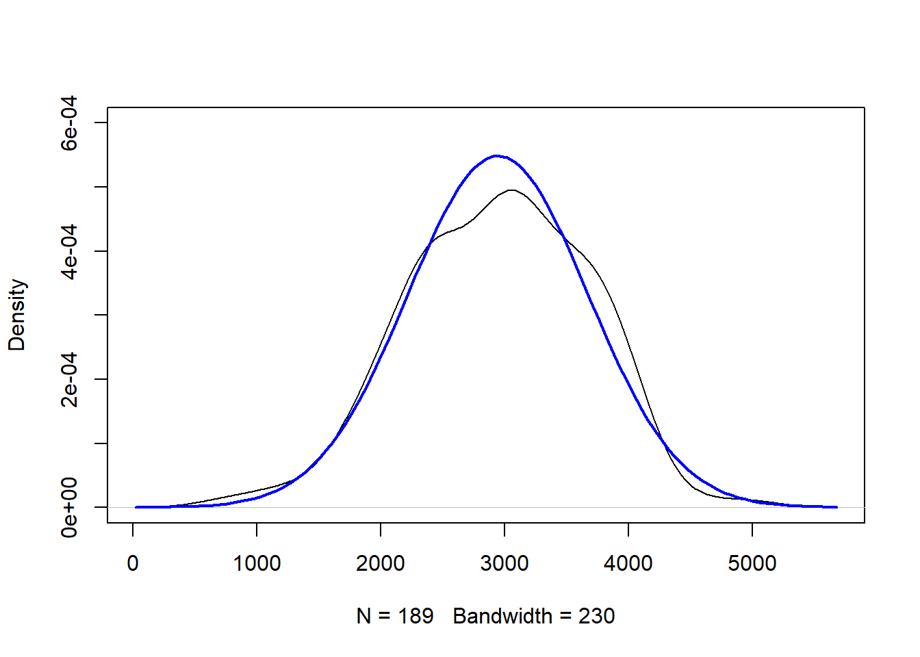

Figure 7.2: Density Plot of Birth Weights. Normal Curve (in Blue) with Parameters Estimated by MOM Overlaid

7.2.1 Alternative Form of Method of Moments Estimation

In Section 4.4.3, we defined central moments. As a reminder, for a random variable \(X\), its \(k\)th central moment is \(E((X-\mu)^k)\).

Suppose we observe a random sample \(x_1, \cdots, x_n\) that comes from \(X\). The \(k\)th sample central moment is \(M_k^* = \frac{1}{n} \sum_{i=1}^n (x_i - \bar{x})^k\).

An alternative form for the method of moments estimation is: Let \(X\) be a random variable with distribution depending on parameters \(\theta_1, \cdots, \theta_m\). The method of moments (MOM) estimates \(\hat{\theta}_1, \cdots, \hat{\theta}_m\) are found by equating the first sample moment to the first moments, and equating subsequent sample central moments to the corresponding central moments, and solving for \(\theta_1, \cdots, \theta_m\).

This alternative form is often easier to work with, since the 2nd central moment is actually the variance of \(X\).

We go back to the 2nd example in the previous subsection, where we are trying to find estimates for \(\mu\) and \(\sigma^2\) of a normal distribution.

• The first moment is \(E(X) = \mu\), since \(X \sim N(\mu, \sigma^2)\).
• The first sample moment is \(M_1 = \frac{1}{n} \sum_{i=1}^n x_i = \bar{x}\).

So we set \(E(X) = M_1\), i.e. \(\hat{\mu} = \bar{x}\). This is just the sample average of the birth weights at Baystate Medical Center in 1986.

• The second central moment is \(Var(x) = E[(X-\mu)^2] = \sigma^2\).
• The second sample central moment is \(M_2^* = \frac{1}{n} \sum_{i=1}^n (x_i - \bar{x})^2\).

So we set \(Var(X) = M_2^*\) i.e. \(\hat{\sigma^2} = \frac{1}{n} \sum_{i=1}^n (x_i - \bar{x})^2\). If we compare this solution with the solution in the previous subsection, they are exactly the same.

The idea behind method of moments estimation is fairly intuitive; however, it has some drawbacks which we will talk about after introducing another method for estimation in the next section, the method of maximum likelihood.

7.3 Method of Maximum Likelihood Estimation

The method of maximum likelihood is a workhorse in statistics and data science since it is widely used in estimating models. It is preferred to the method of moments as it is built upon a stronger theoretical framework, and its estimators tend to have more desirable properties. You are guaranteed to see the method of maximum likelihood again in the future.

As its name suggests, it is a method of estimating parameters by maximizing the likelihood. We will go over the idea behind the likelihood next.

7.3.1 Likelihood Function

Suppose we have \(n\) observations, denoted by the vector \(\boldsymbol{x} = (x_1, \cdots, x_n)^{T}\). We can use a PDF to generalize the distribution of these observations, \(f_{\boldsymbol{X}}(\boldsymbol{x})\). This is a joint PDF of all the variables.

We have seen that PDFs (and hence joint PDFs) are always described by their parameters (e.g. Normal distribution has \(\mu, \sigma^2\), Bernoulli has \(p\)). For this section, we will let \(\boldsymbol{\theta}\) denote the parameters of a PDF. For example, if we are working with multivariate normal distribution, \(\boldsymbol{\theta} = (\boldsymbol{\mu}, \boldsymbol{\Sigma})\), the mean vector and covariance matrix.

We write \(f_{\boldsymbol{X}}(\boldsymbol{x}; \boldsymbol{\theta})\) to express the PDF of the random vector \(\boldsymbol{X}\) with parameter \(\boldsymbol{\theta}\). So the PDF is a function of two items:

• The first item is the vector \(\boldsymbol{x} = (x_1, \cdots, x_n)^{T}\), which is basically a vector of the observed data. In previous modules, we expressed PDFs as a function of the observed data, since we calculate the PDF when \(\boldsymbol{X} = \boldsymbol{x}\). In estimation, the vector of observed data is actually fixed as it is something we are given in the data set.

• The second item is the parameter \(\boldsymbol{\theta}\). Estimating the parameter is our focus in estimation. The general idea in maximum likelihood is to find the value of \(\boldsymbol{\theta}\) that “best explains” or “is most consistent” with the observed values of the data \(\boldsymbol{x}\). We maximize \(f_{\boldsymbol{X}}(\boldsymbol{x}; \boldsymbol{\theta})\) to achieve this goal.

The likelihood function is the PDF, but written in a way that shifts the emphasis to the parameters. The likelihood function is denoted by \(L(\boldsymbol{\theta} | \boldsymbol{x})\) and is defined as \(f_{\boldsymbol{X}}(\boldsymbol{x})\).

Note: the likelihood function should be viewed as a function of \(\boldsymbol{\theta}\), and its shape changes depending on the values of the observed data \(\boldsymbol{x}\).

To simplify calculations involving the likelihood function, we make an assumption that the observations \(\boldsymbol{x}\) are independent and come from an identical distribution with PDF \(f_X(x)\), in other words, the observations are i.i.d. (independent and identically distributed).

Given i.i.d. random variables \(X_1, \cdots, X_n\), each having PDF \(f_X(x)\), the likelihood function is

\[\begin{equation} L(\boldsymbol{\theta} | \boldsymbol{x} ) = \prod_i^n f_X(x; \boldsymbol{\theta}). \tag{7.1} \end{equation}\]

When maximizing the likelihood function, we often log transform the likelihood function first, then maximize the log transformed likelihood function. The log transformed likelihood function is called the log-likelihood function, and it is

\[\begin{equation} \ell(\boldsymbol{\theta} | \boldsymbol{x}) = \log L(\boldsymbol{\theta} | \boldsymbol{x}) = \sum_{i=1}^n \log f_X(x; \boldsymbol{\theta}). \tag{7.2} \end{equation}\]

It turns out that maximizing the log-likelihood function is often easier computationally than maximizing the likelihood function.

As the logarithm is a monotonic increasing function (it never decreases), maximizing a log transformed function is equivalent to maximizing the original function. Next, we look at how to write the likelihood and log-likelihood functions with a couple of examples.

7.3.1.1 Example 1: Bernoulli

Let \(X_1, \cdots, X_n\) be i.i.d. \(Bern(p)\). Find the corresponding likelihood and log-likelihood functions.

From equation (3.8), the PMF of \(X \sim Bern(p)\) is \(f_X(x) = p^x (1-p)^{1-x}\), where the support of \(x\) is \(\{0,1\}\).

The likelihood function, per equation (7.1), becomes

\[ L(p | \boldsymbol{x} ) = \prod_{i=1}^n f_X(x_i; p) = \prod_{i=1}^n p^{x_i} (1-p)^{1-x_i}. \]

The log-likelihood function, per equation (7.2), becomes

\[ \begin{split} \ell (p | \boldsymbol{x}) &= \sum_{i=1}^n \log f_X(x_i;p) \\ &= \sum_{i=1}^n \log \left( p^{x_i} (1-p)^{1-x_i} \right) \\ &= \sum_{i=1}^n x_i \log p + (1-x_i) \log (1-p) \\ &= \log p \left(\sum_{i=1}^n x_i \right) + \log (1-p) \left( n - \sum_{i=1}^n x_i \right). \end{split} \]

7.3.1.2 Example 1 Continued: Visualizing Likelihood and Log-Likelihood Functions

We mentioned that the likelihood and log-likelihood functions, \(L(\boldsymbol{\theta} | \boldsymbol{x} )\) and \(\ell(\boldsymbol{\theta} | \boldsymbol{x} )\), are functions of the parameters \(\boldsymbol{\theta}\) and the observed data \(\boldsymbol{x}\). We typically view these functions after observing our data \(\boldsymbol{x}\).

Suppose we are trying to estimate the proportion of college students who use passphrases for their university email account. We randomly select 20 students and ask them if they use passphrases for their university email account. Let \(x_i\) denote the response for student \(i\), where \(x_i = 1\) if student \(i\) uses passphrases and \(x_i=0\) otherwise. We can say that \(X \sim Bern(p)\) where \(p\) denotes the proportion of all college students who use passphrases for their university email account. For our sample of 20 students, 7 of them said they use passphrases for their university email account. From example 1, we know the likelihood function now is

\[ \begin{split} L(p | \boldsymbol{x} ) &= \prod_{i=1}^n p^{x_i} (1-p)^{1-x_i} \\ &= p^7 (1-p)^{13} \end{split} \]

and the log-likelihood function becomes

\[ \begin{split} \ell (p | \boldsymbol{x}) &= \log p \left(\sum_{i=1}^n x_i \right) + \log (1-p) \left( n - \sum_{i=1}^n x_i \right)\\ &= 7 \log p + 13 \log(1-p). \end{split} \] We can create plots of \(L(p | \boldsymbol{x} )\) and \(\ell(p | \boldsymbol{x} )\) based on the observed data, as we vary the value of \(p\) from 0 to 1 (the support of \(p\)). These plots are displayed in Figure 7.3 below

##function to compute likelihood function 
bern_like<-function(x, p) ##supply vector of data, and value of success probability
  
{
  
  n<-length(x) ##sample size
  S<-sum(x) 
  
  likelihood<-p^S * (1-p)^(n-S) ##formula for likelihood function from Example 1
  return(likelihood)
  
}

##function to compute loglikelihood function

bern_loglike<-function(x,p)
  
{
  
  n<-length(x) ##sample size
  S<-sum(x) 
  
  loglike<- S*log(p) + (n-S)*log(1-p) ##formula for log-likelihood function from Example 1
  return(loglike) 
  
}

##our "data" according to described scenario
data<-c(rep(1,7), rep(0,13)) 
##vary the value of p, from 0 to 1, in increments of 0.01
props<-seq(0,1,by=0.01) 

par(mfrow=c(1,2))
##plot the likelihood function on y axis, against the value of p
plot(props, bern_like(data, props), type="l", xlab="p", ylab="Likelihood Function")
##overlay line on x-axis that corresponds to max value for likelihood function
abline(v=props[which.max(bern_like(data, props))], col="blue")
##plot the loglikelihood function on y axis, against the value of p
plot(props, bern_loglike(data, props), type="l", xlab="p", ylab="Log-Likelihood Function")
##overlay line on x-axis that corresponds to max value for loglikelihood function
abline(v=props[which.max(bern_loglike(data, props))], col="blue")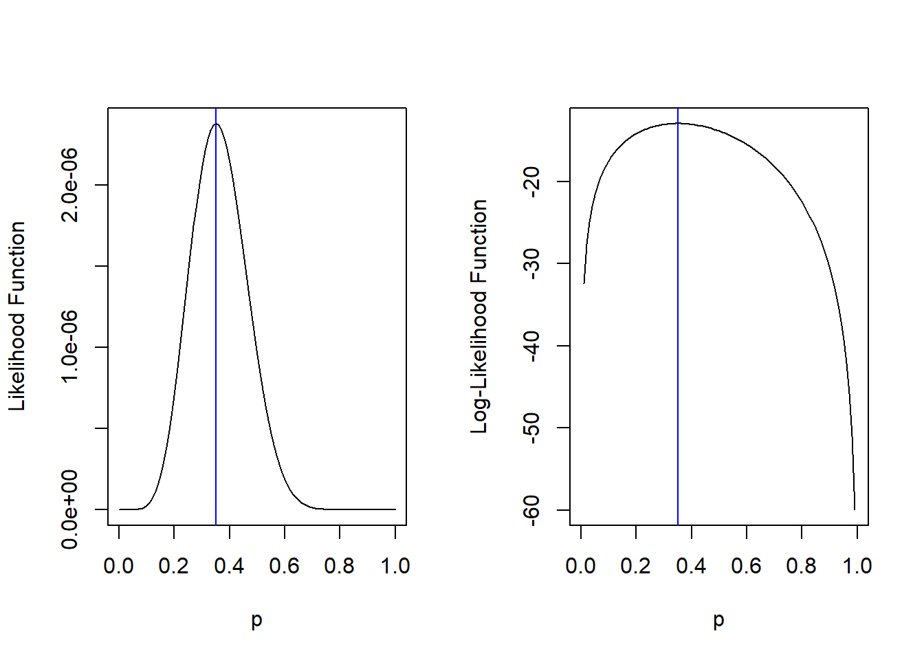

Figure 7.3: Likelihood (left) and Log-Likelihood (right) Functions of Bernoulli, when n=20, and 7 Yeses

## what value of p had maximum value of likelihood
props[which.max(bern_like(data, props))]

## [1] 0.35

## what value of p had maximum value of loglikelihood
props[which.max(bern_loglike(data, props))]

## [1] 0.35

The plots in Figure 7.3 show us how the likelihood and log-likelihood functions behave, given our data (i.e. that 7 out of 20 students said they use passphrases), and as we vary the value of the parameter \(p\). We note that the value of \(p\) that maximized the likelihood and log-likelihood functions is 0.35. This is the idea behind the method of maximum likelihood estimation: what value of the parameter maximizes the likelihood and log-likelihood functions? Or in more regular language, what value of the parameter best explains our data?

Note: the value of 0.35 corresponds to the sample proportion of students who use passphrases. It should make intuitive sense that if 7 out of 20 students in our sample say they use passphrases, we would say that our best estimate for the proportion of college students who use passphrases for their university email is 0.35.

View the video below that provides a bit more detail on finding and visualizing the likelihood and log-likelihood functions for a Bernoulli distribution:

7.3.1.3 Example 2: Normal

Let \(X_1, \cdots, X_n\) be i.i.d. \(N(\mu, \sigma^2)\). Find the corresponding likelihood and log-likelihood functions.

From equation (4.11), the PDF of \(X \sim N(\mu, \sigma^2)\) is \(f_X(x) = \frac{1}{\sigma \sqrt{2 \pi}} \exp \left(-\frac{(x - \mu)^2}{2 \sigma^2} \right)\), where the support of \(x\) is all real numbers.

The likelihood function, per equation (7.1), becomes

\[ L(\mu, \sigma^2 | \boldsymbol{x} ) = \prod_{i=1}^n f_X(x_i; \mu, \sigma^2) = \prod_{i=1}^n \frac{1}{\sigma \sqrt{2 \pi}} \exp \left(-\frac{(x_i - \mu)^2}{2 \sigma^2} \right). \]

The log-likelihood function, per equation (7.2), becomes

\[ \begin{split} \ell (\mu, \sigma^2 | \boldsymbol{x}) &= \sum_{i=1}^n \log f_X(x_i; \boldsymbol{\theta}) \\ &= \sum_{i=1}^n \log \left\{ \frac{1}{\sigma \sqrt{2 \pi}} \exp \left(-\frac{(x_i - \mu)^2}{2 \sigma^2} \right) \right\} \\ &= \sum_{i=1}^n \left\{-\frac{1}{2} \log (2 \pi \sigma^2) -\frac{(x_i - \mu)^2}{2 \sigma^2} \right\} \\ &= -\frac{n}{2} \log (2 \pi \sigma^2) - \frac{1}{2 \sigma^2} \sum_{i=1}^n (x_i - \mu)^2. \end{split} \]

View the video below that provides a bit more detail on finding and visualizing the likelihood and log-likelihood functions for a normal distribution:

7.3.2 Maximum Likelihood Estimation

We are now ready to formally define the method of maximum likelihood estimation. The maximum likelihood (ML) estimates \(\hat{\theta}_1, \cdots, \hat{\theta}_m\) of the parameters \(\theta_1, \cdots, \theta_m\) are found by maximizing the likelihood function \(L(\boldsymbol{\theta} | \boldsymbol{x} )\).

Remember the following when finding ML estimates:

• The values of \(\boldsymbol{x}\) are considered fixed as they are given in our data.
• We are varying the values of the parameters \(\boldsymbol{\theta}\) and finding what specific values of \(\boldsymbol{\theta}\) will maximize the likelihood function.
• We could choose to maximize the log-likelihood function instead. It is often easier to work with the log-likelihood function, as likelihood functions often have exponents (powers) in them, which makes maximizing them more complicated. The solution will be the same.

We re-visit Examples 1 and 2 from the previous subsection.

7.3.2.1 Example 1: Bernoulli

Let \(X_1, \cdots, X_n\) be i.i.d. \(Bern(p)\). Find the ML estimate for \(p\).

We will work with the log-likelihood function, which we had found to be

\[ \ell (p | \boldsymbol{x}) = \log p \left(\sum_{i=1}^n x_i \right) + \log (1-p) \left( n - \sum_{i=1}^n x_i \right). \]

To find the ML estimate for \(p\), we need to find the value of \(p\) that maximizes \(\ell (p | \boldsymbol{x})\). In the previous subsection, we provided a visual way to represent the log-likelihood function as \(p\) is varied, and find the value of \(p\) that corresponded to the peak of the graph. The visual approach only works for a specific scenario when we had 7 out of 20 students who say yes. Can we generalize the ML estimate for the Bernoulli distribution?

We can easily maximize any function by taking its first derivative and setting it to 0. So we take the first derivative of \(\ell (p | \boldsymbol{x})\) with respect to the parameter \(p\):

\[ \begin{split} \frac{d}{d p}\ell (p | \boldsymbol{x}) &= \frac{d}{d p} \left\{ \log p \left(\sum_{i=1}^n x_i \right) + \log (1-p) \left( n - \sum_{i=1}^n x_i \right) \right\}\\ &= \frac{\sum_{i=1}^n x_i}{p} - \frac{n - \sum_{i=1}^n x_i}{1-p} \end{split} \] which we then set to 0:

\[ \begin{split} \frac{\sum_{i=1}^n x_i}{p} - \frac{n - \sum_{i=1}^n x_i}{1-p} &= 0\\ \implies p &= \frac{\sum_{i=1}^n x_i}{n} \end{split} \]

So the ML estimate for \(p\) is \(\hat{p}_{ML} = \frac{\sum_{i=1}^n x_i}{n}\). This is just the sample proportion of observed data where \(x_i = 1\). This result means that for any data that comes from a Bernoulli distribution, the sample proportion of the data that is a “success” is the ML estimate for the success probability \(p\).

If we go back to our example where 7 out of 20 students say they use passphrases, the ML estimate of \(p\) is \(\hat{p}_{ML} = \frac{7}{20} = 0.35\), which matches the result we obtained when we viewed the log-likelihood function visually in Figure 7.3.

View the video below that provides a bit more detail on deriving the ML estimates for a Bernoulli distribution:

Thought question: Play around with the code that produced Figure 7.3. Change the vector data (to anything you’d like). You should find that the value of \(p\) that maximizes the likelihood and log-likelihood functions will always be \(\hat{p}_{ML} = \frac{\sum_{i=1}^n x_i}{n}\), the sample proportion of “success” in our sample.

7.3.2.2 Example 2: Normal

Let \(X_1, \cdots, X_n\) be i.i.d. \(N(\mu, \sigma^2)\). Find the ML estimates for \(\mu\) and \(\sigma^2\).

Again, we will work with the log-likelihood function, which we had found to be

\[ \ell (\mu, \sigma^2 | \boldsymbol{x}) = -\frac{n}{2} \log (2 \pi \sigma^2) - \frac{1}{2 \sigma^2} \sum_{i=1}^n (x_i - \mu)^2. \]

Notice we have two parameters \(\mu\) and \(\sigma^2\), so we have to take partial derivatives \(\ell (\mu, \sigma^2 | \boldsymbol{x})\) for with respect to each parameter:

• Partial derivative with respect to \(\mu\):

\[ \begin{split} \frac{d}{d \mu}\ell (\mu, \sigma^2 | \boldsymbol{x}) &= \frac{d}{d \mu} \left\{ -\frac{n}{2} \log (2 \pi \sigma^2) - \frac{1}{2 \sigma^2} \sum_{i=1}^n (x_i - \mu)^2 \right \} \\ &= \frac{1}{\sigma^2} \sum_{i=1}^n (x_i - \mu). \end{split} \]

• Partial derivative with respect to \(\sigma^2\):

\[ \begin{split} \frac{d}{d \sigma^2}\ell (\mu, \sigma^2 | \boldsymbol{x}) &= \frac{d}{d \sigma^2} \left\{ -\frac{n}{2} \log (2 \pi \sigma^2) - \frac{1}{2 \sigma^2} \sum_{i=1}^n (x_i - \mu)^2 \right \} \\ &= -\frac{n}{2}\frac{2\pi}{2 \pi \sigma^2} + \frac{1}{2 \sigma^4} \sum_{i=1}^n (x_i - \mu)^2 \\ &= -\frac{n}{2 \sigma^2} + \frac{1}{2 \sigma^4} \sum_{i=1}^n (x_i - \mu)^2 \end{split} \] We then set both partial derivatives to 0:

\[ \begin{split} \frac{d}{d \mu}\ell (\mu, \sigma^2 | \boldsymbol{x}) &= 0 \\ \implies \frac{1}{\sigma^2} \sum_{i=1}^n (x_i - \mu) &= 0 \\ \implies \mu &= \frac{\sum_{i=1}^n x_i}{n} = \bar{x}. \end{split} \] So the ML estimate for \(\mu\) is \(\hat{\mu_{ML}} = \bar{x}\), i.e. the sample mean.

\[ \begin{split} \frac{d}{d \sigma^2}\ell (\mu, \sigma^2 | \boldsymbol{x}) &= 0 \\ \implies -\frac{n}{2 \sigma^2} + \frac{1}{2 \sigma^4} \sum_{i=1}^n (x_i - \mu)^2 &= 0 \\ \implies \sigma^2 &= \frac{\sum_{i=1}^n (x_i - \mu)^2}{n}. \end{split} \]

So the ML estimate for \(\sigma^2\) is \(\hat{\sigma_{ML}^2} = \frac{\sum_{i=1}^n (x_i - \mu)^2}{n}\). Note that this is not the same as how we normally calculate sample variance, per equation (1.2): \(\frac{\sum_{i=1}^n (x_i-\bar{x})^2}{n-1}\).

View the video below that provides a bit more detail on deriving the ML estimates for a normal distribution:

7.3.2.3 Calculating Maximum Likelihood Estimates

In the examples that we have worked with, we found the values of maximum likelihood estimates using a couple of approaches, one using a plot of the likelihood function over different values of the parameter, based on observed data, and another using calculus, by setting the derivative of the log-likelihood function to 0.

There are times when these approaches may not be feasible, for example, there is no closed form solution for the first derivative. In these instances, numerical methods are used. Numerical methods are typically algorithms that perform complex computations to approximate a mathematical result. We will not go into the details of these algorithms, and numerical methods are still an active area of research.

7.4 Properties of Estimators

We have learned about a couple of different methods to estimate parameters. While these two methods are common, there are not the only methods to estimate parameters. One question how do we assess if our estimates are “good” or not? We define a few concepts that are used in this assessment.

7.4.1 Estimators VS Estimates

We wrote about estimators and estimates earlier in this module, but as a quick reminder on what these are:

• An estimator is a numerical summary associated with samples.

• An estimated value, or estimate, is the actual value of the estimator based on a sample.

We have previously said that the ML estimate is found by maximizing the likelihood function, i.e. \(\hat{\theta}_{ML}(\boldsymbol{x})\) is the value of \(\theta\) that maximizes \(L(\theta| \boldsymbol{x})\). We write \(\hat{\theta}_{ML}(\boldsymbol{x})\) to emphasize that the ML estimate is a function of the observed data \(\boldsymbol{x} = (x_1,\cdots, x_n)^T\). So, if our ML estimate is the sample mean, we write \(\hat{\theta}_{ML}(\boldsymbol{x}) = \frac{\sum_{i=1}^n x_i}{n}\). This value is calculated based on our observed data. We can also view the sample mean as a random variable, especially if we want to analyze the uncertainty associated with the sample mean. In other words, what is the distribution of the sample mean, if we had obtained many different random samples and calculated the sample mean from each random sample? When viewing the sample mean as a random variable, we write \(\hat{\Theta}_{ML}(\boldsymbol{X}) = \frac{\sum_{i=1}^n X_i}{n}\), and we call \(\hat{\Theta}_{ML}\) the ML estimator of the parameter \(\theta\).

Note: we consider one parameter \(\theta\) in this subsection, to simplify notation with the introduction of \(\Theta\). The ideas can be applied to any number of parameters.

The ML estimators are just one kind of estimators. We can find estimators in other ways (method of moments, or any other method). An estimator is any function that uses the data and calculates a number from the data and can be denoted as \(\hat{\Theta}(\boldsymbol{X})\). We call \(\hat{\Theta}\) an estimator of \(\theta\).

Consider \(X_1, \cdots, X_n\) i.i.d. Normal with unknown mean \(\mu\) and variance \(\sigma^2\) that is known. We can define two estimators of \(\mu\) as \(\hat{\Theta}_1(\boldsymbol{X}) = \frac{\sum_{i=1}^n X_i}{n}\) and \(\hat{\Theta}_2(\boldsymbol{X}) = X_1 + 2\). The first estimator takes the average value of the \(n\) data points. The second estimator uses the first data point and adds 2 to it. The first estimator is an ML estimator, while the second estimator is not.

We can see that we are free to define estimators in various ways. The question now is how do we evaluate whether an estimator is “good” or not. There are a few metrics to evaluate estimators.

7.4.2 Bias

One metric used to evaluate estimators is to consider the long-run average of an estimator. An estimator is unbiased if the long run average of an estimator is equal to the true value of the parameter. Mathematically, an estimator \(\hat{\Theta}\) is unbiased if \(E(\hat{\Theta}) = \theta\). From this definition of an unbiased estimator, we have the definition of the bias of an estimator:

\[\begin{equation} Bias(\hat{\Theta}) = E(\hat{\Theta}) - \theta. \tag{7.3} \end{equation}\]

So, while the value of the estimator could vary from sample to sample, the estimator is unbiased if it is equal to the true parameter, on average in the long-run.

We go back to the example from the previous subsection. Consider \(X_1, \cdots, X_n\) i.i.d. Normal with unknown mean \(\mu\) and variance \(\sigma^2\) that is known. we can define two estimators of \(\mu\) as \(\hat{\Theta}_1(\boldsymbol{X}) = \frac{\sum_{i=1}^n X_i}{n}\) and \(\hat{\Theta}_2(\boldsymbol{X}) = X_1 + 2\). Assess whether \(\hat{\Theta}_1(\boldsymbol{X})\) and \(\hat{\Theta}_2(\boldsymbol{X})\) are unbiased or not.

• The mathematical way of answering this question is to evaluate the expected value of both estimators:

  • \(E(\hat{\Theta}_1) = \frac{1}{n}E(\sum_{i=1}^n X_i) = \frac{1}{n}\sum_{i=1}^n E(X_i) = \frac{1}{n}(\mu + \cdots + \mu) = \mu\), so it is unbiased.

  • \(E(\hat{\Theta}_2) = E(X_1 + 2) = E(X_1) + 2 = \mu +2\) which is not equal to \(\mu\), so it is biased.

• We can also use Monte Carlo simulations to show these results. The simulation should do the following:

  • The code simulates \(X_1, \cdots, X_{n}\) i.i.d. from a known distribution, and with \(n\) fixed. In the code below, I used a standard normal, with \(n=100\).
    
  • Generate a large number of replicates (I used 10 thousand replicates) of \(X_1, \cdots, X_{n}\).
  • For each replicate of \(X_1, \cdots, X_{n}\), calculate \(\hat{\Theta}_1(\boldsymbol{X}) = \frac{\sum_{i=1}^n X_i}{n}\) and \(\hat{\Theta}_2(\boldsymbol{X}) = X_1 + 2\).
  • We then find the average of \(\hat{\Theta}_1(\boldsymbol{X})\) and \(\hat{\Theta}_2(\boldsymbol{X})\) across the replicates.

If the estimator is unbiased, the average from the Monte Carlo simulation should be close to 0, since the true mean of a standard normal is 0.

reps<-10000

est1<-est2<-array(0,reps) ##array to store est1 & est2 from each rep

n<-100

set.seed(7)

for (i in 1:reps)
  
{
  
  X<-rnorm(n) ##Xi iid N(0,1) with n=100
  
  est1[i]<-mean(X) ##est 1
  est2[i]<-X[1] + 2 ##est 2
  
}

mean(est1) ##should be close to 0, indicating sample mean is unbiased

## [1] -0.0009093132

mean(est2) ##should not be close to 0, indicating first obs + 2 is biased

## [1] 2.003234

##create density plots to show distribution for est1 and est 2, and overlay line to show true value of mu
par(mfrow=c(1,2))
plot(density(est1), main="Density Plot for Theta1")
abline(v=0, col="blue")
plot(density(est2), main="Density Plot for Theta2")
abline(v=0, col="blue")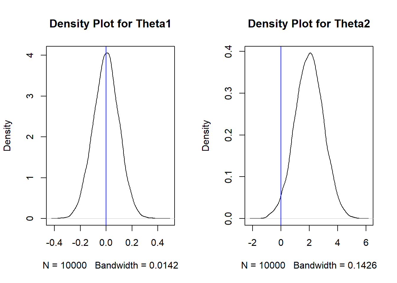

Figure 7.4: Dist of Theta1 (left) and Theta2 (right)

Figure 7.4 displays the distribution of the 10 thousand \(\hat{\Theta}_1(\boldsymbol{X})\)s and \(\hat{\Theta}_2(\boldsymbol{X})\)s. Visually, an estimator is unbiased if its “middle” is equal to the value of the parameter, which is 0. We can see this is clearly not the case for \(\hat{\Theta}_2(\boldsymbol{X})\) so it is biased.

The results from the MC simulation matches with the math. We had shown that \(\hat{\Theta}_1(\boldsymbol{X}) = \frac{\sum_{i=1}^n X_i}{n}\) is an unbiased estimator for \(\mu\), whereas \(\hat{\Theta}_2(\boldsymbol{X}) = X_1 + 2\) is a biased estimator.

So, based on bias, the sample mean is a better estimator for the population mean than using the first data point and adding 2 to it.

The bias deals with the centrality of the estimator, i.e. is the estimator equal to the true parameter, on average. As we have seen in previous modules, we are not only concerned with measures of centrality, but also with measures of uncertainty. For example, how likely is it to observe a random sample where its estimated value is far from the true parameter?

7.4.3 Standard Error and Variance

It turns out that the concept of variance can also be applied to estimators, as they can be viewed as random variables, and not just to individual data points. Estimators with smaller variances have a smaller degree of uncertainty: the value of the estimators do not change as much from random sample to random sample.

We can go back to the example from the previous subsection. Consider \(X_1, \cdots, X_n\) i.i.d. Normal with unknown mean \(\mu\) and variance \(\sigma^2\) that is known. We defined two estimators of \(\mu\) as \(\hat{\Theta}_1(\boldsymbol{X}) = \frac{\sum_{i=1}^n X_i}{n}\) and \(\hat{\Theta}_2(\boldsymbol{X}) = X_1 + 2\). Derive the variance of both estimators.

The mathematical way of answering this question is to evaluate the variance of both estimators:

• \(Var(\hat{\Theta}_1) = \frac{1}{n^2}Var(\sum_{i=1}^n X_i) = \frac{1}{n^2} \sum_{i=1}^n Var(X_i) = \frac{1}{n^2} (\sigma^2 + \cdots + \sigma^2) = \frac{\sigma^2}{n}\).

• \(Var(\hat{\Theta}_2) = Var(X_1 + 2) = Var(X_1) = \sigma^2\).

There is also a separate term used when evaluating the variance of an estimator: this is the standard error of an estimator. This is essentially the standard deviation of the estimator, i.e. \(SE(\hat{\Theta}) = \sqrt{Var(\hat{\Theta})}\). Going back to our example: \(SE(\hat{\Theta}_1) = \frac{\sigma}{\sqrt{n}}\) and \(SE(\hat{\Theta}_2) = \sigma\).

Note: The term standard error is only applied to estimators. It is not used when finding the standard deviation of data points.

We can also use our Monte Carlo simulation from the previous subsection to estimate these values:

var(est1) ##should be close to 1/100, since n=1000

## [1] 0.009956095

var(est2) ##should be close to 1

## [1] 0.9988228

sd(est1) ##should be close to 1/10

## [1] 0.09978023

sd(est2) ##should be close to 1

## [1] 0.9994112

These results are reflected in Figure 7.4. Notice the scale of the x-axis for the plot of \(\hat{\Theta}_2\) (on the right) is much larger, so \(\hat{\Theta}_2\) has larger variability than \(\hat{\Theta}_1\), i.e. we are more uncertain about the value of \(\hat{\Theta}_2\), since they deviate more from each other.

It should be clear by now that estimators with smaller standard errors (or variances) are desired. So, based on standard error, the sample mean is a better estimator for the population mean than using the first data point and adding 2 to it.

7.4.3.1 Consistency

An associated concept with variance and standard errors of estimators is consistency. The definition of consistency in estimators is fairly technical, so we will give a broad overview of its concept.

Notice how we have denoted an estimator as \(\hat{\Theta}(\boldsymbol{X})\), where \(\boldsymbol{X} = (X_1, \cdots, X_n)^T\). So it stands to reason that the behavior of \(\hat{\Theta}(\boldsymbol{X})\) may change as the number of data points \(n\) changes. We will use the notation \(\hat{\Theta}_n\) to denote an estimator that is based on \(n\) data points, to emphasize that we are focusing on how the estimator changes as \(n\) changes.

An estimator is consistent if \(\hat{\Theta}_n\) gets closer to and approaches the true value of \(\theta\) as \(n\) gets larger and approaches infinity. This means as the sample size \(n\) gets larger, the estimator tends to get closer to the true value of the parameter.

We go back to the example from the previous subsection. Consider \(X_1, \cdots, X_n\) i.i.d. Normal with unknown mean \(\mu\) and variance \(\sigma^2\) that is known. We defined two estimators of \(\mu\) as \(\hat{\Theta}_1(\boldsymbol{X}) = \frac{\sum_{i=1}^n X_i}{n}\) and \(\hat{\Theta}_2(\boldsymbol{X}) = X_1 + 2\). Assess whether \(\hat{\Theta}_1(\boldsymbol{X})\) and \(\hat{\Theta}_2(\boldsymbol{X})\) are consistent or not.

• The mathematical way of answering this question involves a few more mathematical concepts that we will not get into. A general way of assessing if an estimator is consistent is to see if its variance shrinks towards zero as \(n\) gets larger and goes to infinity.

  • We had earlier showed that \(Var(\hat{\Theta}_1) = \frac{\sigma^2}{n}\), which shrinks towards zero as \(n\) gets larger, so it is consistent.

  • We had earlier showed that \(Var(\hat{\Theta}_2) = \sigma^2\), which does not shrink towards zero as \(n\) gets larger, so it is not consistent.

• We can also use Monte Carlo simulations to show these results:

  • The code simulates \(X_1, \cdots, X_{n}\) i.i.d. from a known distribution, and with \(n\) varied from small values to large values. In the code below, I used a standard normal, with \(n=10, 100, 1000\).
    
  • For each value of \(n\), generate a large number of replicates (I used 10 thousand replicates) of \(X_1, \cdots, X_{n}\).
  • For each replicate of \(X_1, \cdots, X_{n}\), calculate \(\hat{\Theta}_1(\boldsymbol{X}) = \frac{\sum_{i=1}^n X_i}{n}\) and \(\hat{\Theta}_2(\boldsymbol{X}) = X_1 + 2\).
  • We then produce density plots of \(\hat{\Theta}_1\) and \(\hat{\Theta}_2\) when \(n=10, 100, 1000\).

If an estimator is consistent, we should notice the spread of its density plot get narrower as \(n\) gets larger.

n<-c(10,100,1000)

reps<-10000

est1<-est2<-array(0,c(length(n),reps)) ##arrays to store est 1 and est 2 as n changes

set.seed(50)

for (i in 1:length(n))
  
{
  
  for (j in 1:reps)
    
  {
    
    X<-rnorm(n[i])
    est1[i,j]<-mean(X) ##est 1
    est2[i,j]<-X[1]+2 ##est 2
    
  }
  
}

par(mfrow=c(1,2))

##find max value of density plots for est 1 so plots all show up complete
max_y1 <- max(density(est1[1,])$y, density(est1[2,])$y, density(est1[3,])$y) 

plot(density(est1[1,]), ylim=c(0, max_y1), main="Density Plot of Est1 with n Varied")
lines(density(est1[2,]), col="blue")
lines(density(est1[3,]), col="red")
legend("topright", legend = c("n=10", "n=100", "n=1000"), col = c("black","blue", "red"), lty = 1, cex=0.7)

##find max value of density plots for est 2 so plots all show up complete
max_y2 <- max(density(est2[1,])$y, density(est2[2,])$y, density(est2[3,])$y)

plot(density(est2[1,]), ylim=c(0, max_y2), main="Density Plot of Est2 with n Varied")
lines(density(est2[2,]), col="blue")
lines(density(est2[3,]), col="red")
legend("topright", legend = c("n=10", "n=100", "n=1000"), col = c("black","blue", "red"), lty = 1, cex=0.7)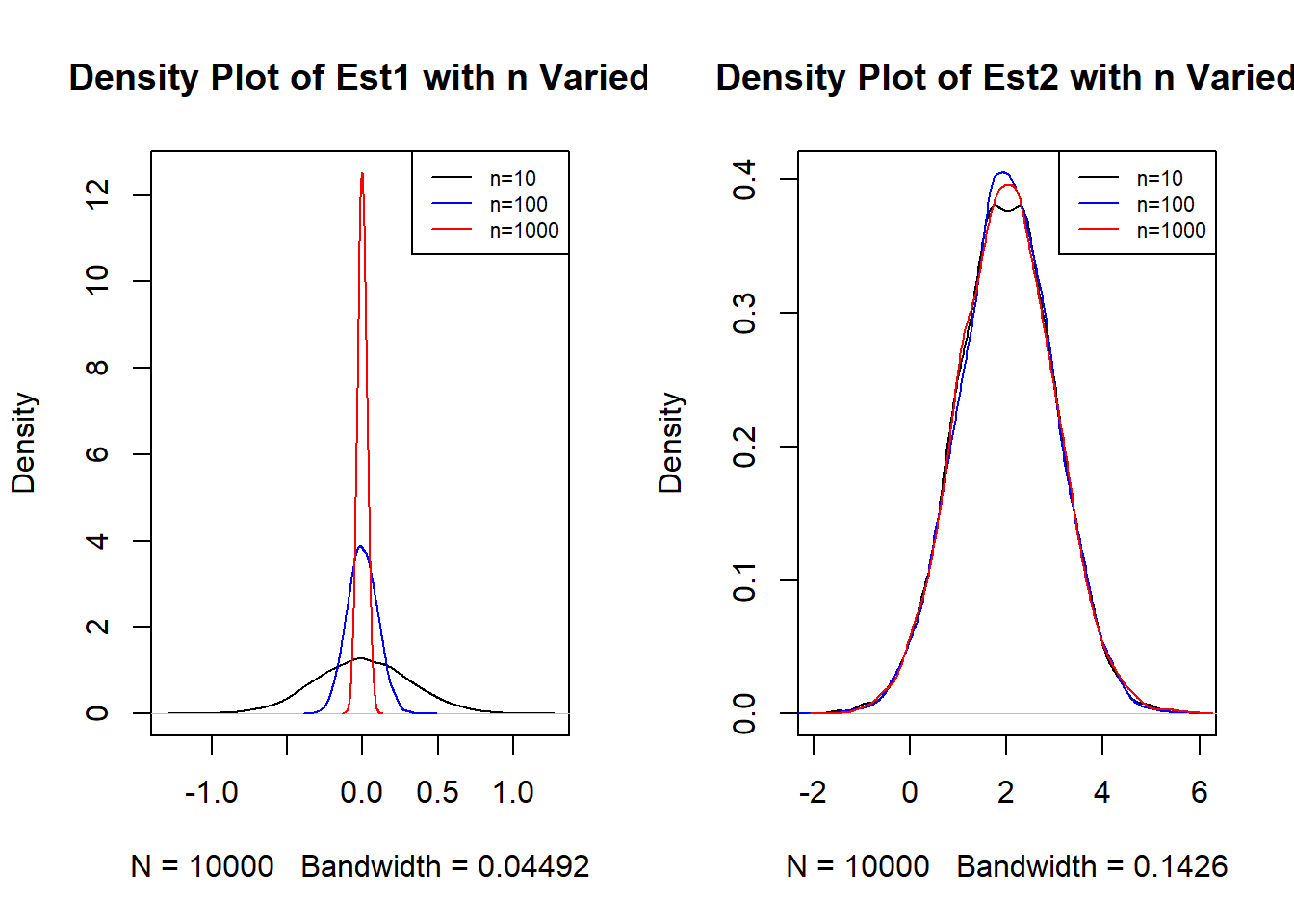

Figure 7.5: Dist of Theta1 (left) and Theta2 (right) as n is Varied

Figure 7.5 displays the distribution of the 10 thousand \(\hat{\Theta}_1(\boldsymbol{X})\)s and \(\hat{\Theta}_2(\boldsymbol{X})\)s when \(n=10, 100, 1000\). Visually, an estimator is consistent if its density plot becomes narrower as \(n\) gets larger. We see this in the left plot, so \(\hat{\Theta}_1(\boldsymbol{X})\) is consistent, but we do not see this in the right plot, so \(\hat{\Theta}_2(\boldsymbol{X})\) is not consistent.

Note that unbiased estimators and consistent estimators are two different concepts. An estimator could be unbiased but inconsistent, or it could be biased but consistent.

Thought question: Suppose \(X_1, \cdots, X_n\) i.i.d. standard normal. Consider an estimator for \(\mu\), \(\hat{\Theta}_3 = X_1\), and an estimator for \(\sigma^2\), \(\hat{\Theta}_4 = \frac{1}{n} \sum_{i=1}^n (X_i - \mu)^2\). The book says that \(\hat{\Theta}_3\) is an unbiased but inconsistent estimator for \(\mu\), and \(\hat{\Theta}_4\) is a biased but consistent estimator for \(\sigma^2\). Can you use Monte Carlo simulations to verify these claims?

7.4.4 Sampling Distribution

The plots in Figure 7.4 and Figure 7.5 give rise to the idea that there is a distribution associated with an estimator. There is a term for this, called the sampling distribution of an estimator.

Some estimators have known distributions, for example the sample mean, \(\bar{X}\). Some other common estimators also have known distributions, such as the sample proportion as an estimator for the population proportion, the sample variance as an estimator for the population variance, as well as ML estimators for linear regression and logistic regression models.

If the sampling distribution of an estimator is known and follows well known distributions, we can easily perform probability calculations involving estimators, for example, how likely are we to observe a sample mean that is more than 2 standard errors away from its true mean?

However, other estimators may not have known distributions, for example, the sample median as an estimator for the population median has no known sampling distribution. Does this mean that we are unable to calculate probabilities associated with such estimators? It turns out there exist methods called resampling methods that allow us to approximate these calculations. We will cover the bootstrap, which is a commonly used resampling method, in a future module.

7.4.4.1 Sampling Distribution of Sample Mean

We will state the sampling distribution of the sample mean, \(\bar{X}_n\). There are a couple of conditions to consider:

1. \(X_1, \cdots, X_n\) are i.i.d. from a normal distribution with finite mean \(\mu\) and finite variance \(\sigma^2\). Then \(\bar{X}_n \sim N(\mu, \frac{\sigma^2}{n})\). This result is based on the fact that the sum of independent normals result in a normal distribution.

This means that if the data are originally normally distributed, the sample mean will be normally distributed, regardless of the sample size.

2. \(X_1, \cdots, X_n\) are i.i.d. from any distribution with finite mean \(\mu\) and finite variance \(\sigma^2\), and if \(n\) is large enough, then \(\bar{X}_n\) is approximately \(N(\mu, \frac{\sigma^2}{n})\). This is based on the CLT in section 6.3.2.

This means that even if the data are not originally normally distributed, the sample mean will be approximately normally distributed if the sample size is large enough.

We apply the sampling distribution of the sample mean to the left plot in Figure 7.5, which visually displays the distribution of the sample mean with \(n=10, 100, 1000\). The data were i.i.d. standard normal, so we meet the first scenario and know that the sample means follow a normal distribution:

• When \(n=10\), \(\bar{X}_n \sim N(0, \frac{1}{10}) = N(0, 0.1)\).
• When \(n=100\), \(\bar{X}_n \sim N(0, \frac{1}{100}) = N(0,0.01)\).
• When \(n=1000\), \(\bar{X}_n \sim N(0, \frac{1}{1000}) = N(0,0.001)\).

We see that when the sample size gets larger, the variance of the sample mean decreases, so there is less spread and their resulting density plot is more concentrated around the mean. This matches with what we see in the left plot in Figure 7.5.

7.4.5 Mean-Squared Error

We introduced the mean-squared error (MSE) in the context of evaluating prediction errors in Section 4.4.1.3. The MSE can also be used to evaluate an estimator. In this context, the MSE of an estimator \(\hat{\Theta}\) is

\[\begin{equation} MSE(\hat{\Theta}) = E\left[(\hat{\Theta} - \theta)^2 \right]. \tag{7.4} \end{equation}\]

The MSE of an estimator can be interpreted as the average squared difference between an estimator and the value of its parameter. It turns out that the MSE of an estimator is related to two other metrics: the bias of an estimator and the variance of an estimator:

\[\begin{equation} MSE(\hat{\Theta}) = Var(\hat{\Theta}) + Bias(\hat{\Theta})^2. \tag{7.5} \end{equation}\]

In other words, the MSE of an estimator is equal to the variance of an estimator plus the squared bias of an estimator. Equation (7.5) is often called the bias-variance decomposition of the MSE. If an estimator is unbiased, equation Equation (7.5) tells us that the MSE of an estimator is equal to its variance.

What the MSE of an estimator suggests is that we need to consider both the bias and variance of an estimator. People often think that an unbiased estimator is the “best”. However, an unbiased estimator could have high variance. Such an estimator could have high MSE. In such a setting, it may be worth considering another estimator that may be biased, but have much smaller variance, resulting in a lower MSE. An example of where this can happen is in linear regression. Classical methods with linear regression yield unbiased estimators, but under specific scenarios, these estimators could have high variances. Another model, called the ridge regression model, considers biased estimators which may have smaller variances, which can result in lower MSEs in these specific scenarios. You will learn about these models in greater detail in a future class.

7.5 Final Comments on Estimation

We have covered the method of moments and method of maximum likelihood when estimating parameters. These methods are also called parametric methods as they involve making an assumption that the data follow some well-known distribution with unknown parameters, and we are then using our data, and our assumed distribution, to estimate the numerical value of the unknown parameters.

There exist nonparametric methods in estimation. We have actually seen one such method (without calling it nonparametric), which is kernel density estimation (KDE) in Section 4.6.1. KDE is used to estimate the PDF of a random variable so that we can visualize its distribution. If you look back at KDE, you will notice we made no assumption about the distribution of the random variable. This is one of the fundamental differences between parametric and nonparametric estimation: the former assumes a distribution for the data, the latter does not.

7.5.1 Why ML Estimators?

I had mentioned earlier that ML estimators are considered the workhorse in statistics and data science and is likely the most common type of estimator used. ML estimators have these properties:

• ML estimators are consistent.
• ML estimators are asymptotically Normal, i.e. \(\frac{\hat{\Theta} - \theta}{SE(\hat{\Theta})}\) is approximately standard normal as \(n\) approaches infinity. This also implies that ML estimators are asymptotically unbiased, i.e. for large \(n\), the bias shrinks towards 0.
• ML estimators are efficient. As \(n\) approaches infinity, ML estimators have lowest variance among all unbiased estimators. However, for smaller sample sizes, ML estimators may be biased and so other unbiased estimators could have smaller variances.
• ML estimators are equivariant. If \(\hat{\Theta}\) is the ML estimator of \(\theta\), then \(g(\hat{\Theta})\) is the ML estimator for \(g(\theta)\).

What these properties imply is that if your sample size is large enough, estimates from ML estimators are highly likely to be close to the value of the parameter, ML estimators are virtually unbiased, are approximately normally distributed, and have the smallest variance among other possible unbiased estimators. These properties do not exist when the sample size is small.

The MOM estimators do not necessarily have these properties.

These properties require what are called regularity conditions. The definitions get fairly technical and are beyond the scope of the class. One of the conditions is that the data have to be i.i.d..