8 Categorical Predictors in MLR

8.1 Introduction

Thus far, we have only considered predictors that are quantitative in MLR. But what if we need or want to consider predictors that are categorical instead? For example, what if we wish to investigate the earnings of college graduates based on the type of major? The predictor variable, type of major, is clearly categorical and not quantitative. Categorical variables can be incorporated in MLR. In this module, you will learn how to use and interpret the MLR model when categorical predictors are present.

8.1.1 Quantitative vs categorical variable

First, a quick review on variable types. Variables can be divided into two types: quantitative or categorical. A general way to assess the type of a variable is the answer to the following question: Do arithmetic operations on the variable make sense? If yes, the variable is quantitative.

8.1.1.1 Quantitative variable

Quantitative variables are measured in terms of numbers, where the number represents an amount. Quantitative variables can be subdivided into either continuous or discrete.

• Continuous quantitative variable: takes on any numerical value within a range. E.g.: height can be measured in terms of centimeters or inches. It is continuous as the value can take on any value between the shortest and tallest person.
• Discrete quantitative variable: takes on distinct numerical values. E.g. the number of failures among 10 experiments. It is discrete as it can only take on integers between 0 and 10.

A question to determine if the variable is continuous or discrete: Can you potentially list all the plausible values of the variable? If yes, the variable is discrete. For the example above, we can list the plausible values for the number of failures among 10 experiments as: 0, 1, 2, all the way to 10. For the height variable, the list of numerical values for height will be an infinite list as height can take on an infinite number of decimal places.

8.1.1.2 Categorical variables

Categorical variables express qualitative attributes (often called qualitative variable). The levels (or classes) are the various attributes the variable can take on. For example, political affiliation is categorical with three levels: Democrat, Republican, Independent.

A binary variable is a categorical variable with two levels. For example, a variable on whether you voted during the 2020 presidential election is binary, as the answer is either yes or no.

The choice of methods used to analyze data are usually driven by whether the variables are quantitative or categorical. You might have noticed this when creating data visualizations: the visualization you use is driven by the type of variable. Discrete variables are interesting since we can use methods meant for quantitative or categorical variables. We will go over how to make this decision in the context of building MLR models later in the module.

We will see how to incorporate categorical predictors in MLR. We will first start with binary predictors before moving on to predictors with more than two levels.

8.2 Indicator Variables and Dummy Coding

Let us start by considering this simple example: In a study of innovation in the insurance industry, an economist wishes to relate the speed with which an insurance innovation is adopted (in months), \(y\), to the size of the firm, \(x_1\), and the type of firm (mutual or stock firms).

Data<-read.table("insurance.txt", header=FALSE,sep="")
colnames(Data)<-c("time","size", "firm")
head(Data)

##   time size   firm
## 1   17  151 mutual
## 2   26   92 mutual
## 3   21  175 mutual
## 4   30   31 mutual
## 5   22  104 mutual
## 6    0  277 mutual

So we have one categorical variable, the type of firm, that is binary, as it has two levels, mutual or stock. We also have a quantitative predictor, the size of the firm, \(x_1\), and a quantitative response variable, the time to adopt an innovation.

8.2.1 Indicator variables

Indicator variables that take on the values 0 and 1 are commonly used to represent the levels of categorical predictors. For example, we may have the following two indicator variables to represent the two types of firms:

\[\begin{eqnarray*} x_2 &=& \left\{ \begin{array}{ll} 1 & \mbox{ if mutual firm} \\ 0 & \mbox{ otherwise;} \end{array}\right. \\ x_3 &=& \left\{ \begin{array}{ll} 1 & \mbox{ if stock firm} \\ 0 & \mbox{ otherwise;} \end{array} \right. \end{eqnarray*}\]

and the MLR model is written as \[ y_i = \beta_0 + \beta_1x_{i1} + \beta_2x_{i2} + \beta_3x_{i3} + \epsilon_i. \] However, this will not work in MLR. Recall that the least squares estimators are

\[\begin{equation} \boldsymbol{\hat{\beta}} = \left(\boldsymbol{X}^{\prime} \boldsymbol{X} \right)^{-1} \boldsymbol{X}^{\prime} \boldsymbol{y} . \tag{8.1} \end{equation}\]

The matrix \((\boldsymbol{X}^{\prime} \boldsymbol{X})\) is not invertible if we use these indicator variables. Let us consider a toy example where \(n=4\), with the first two observations being mutual fims, and the last two observations being stock furms. The design matrix, \(\boldsymbol{X}\), becomes

\[ \left[ \begin{array}{cccc} 1 & x_{11} & 1 & 0 \\ 1 & x_{21} & 1 & 0 \\ 1 & x_{31} & 0 & 1 \\ 1 & x_{41} & 0 & 1 \\ \end{array} \right] \] Notice that in the design matrix, column 1 equals to the sum of column 3 and column 4. This means we have linear dependence among the columns of the design matrix. And when this happens, \((\boldsymbol{X}^{\prime} \boldsymbol{X})^{-1}\) cannot be found so unique solutions to the least squares estimators (8.1) do not exist.

To get around this issue, we use what is known as dummy coding.

8.2.2 Dummy coding

We drop one of the indicator variables. In general, a categorical variable with \(a\) levels will be represented by \(a-1\) indicator variables, each taking on the values of 0 and 1. This method of coding categorical variables is called dummy coding. So for our example, since firm type is binary (two levels), we only need one indicator variable.

We can have the following model

\[\begin{equation} y = \beta_0 + \beta_1x_{1} + \beta_2I_{1} + \epsilon, \tag{8.2} \end{equation}\]

where \(x_1=\) is the size of the firm and

\[\begin{eqnarray*} I_1 &=& \left\{ \begin{array}{ll} 1 & \mbox{ if stock firm} \\ 0 & \mbox{ otherwise.} \end{array}\right. \end{eqnarray*}\]

So in this formulation, we only use one indicator variable, \(I_1\). Indicator variables are typically denoted by \(I\). In this formulation, mutual firm is coded 0, and stock firm is coded 1. The level that is coded 0 is called the reference class (sometimes called the baseline class). When the variable is binary, the choice for reference class is not important. The interpretation of the model does not change based on the choice for the reference class.

8.2.3 Regression coefficient interpretation

To see how we can interpret the regression coefficients with dummy coding, we can substitute the numerical value of the indicator variable in (8.2) to obtain the regression equation for each firm type:

• Mutual firms: \(E(y|x) = \beta_0 + \beta_1x_1 +\beta_2(0) = \beta_0 + \beta_1x_1\)

• Stock firms: \(E(y|x) = \beta_0 + \beta_1x_1 + \beta_2(1) = (\beta_0+\beta_2) + \beta_1x_1\)

We make the following observations:

• We have two straight lines, with the same slope \(\beta_1\), but the intercepts are different, \(\beta_0\) and \(\beta_0 + \beta_2\). This formulation assumes the slope in the scatterplot of \(y\) against \(x_1\) is the same for both firm types.
• \(\beta_2\) indicates the difference in the mean response for stock firms versus mutual firms (stock firms minus mutual firms), when controlling for size of firm.

In general, the coefficient of an indicator variable shows how much higher (or lower) the mean response is for the class coded 1 than the reference class, when controlling for \(x_1\).

Let us look at our example:

##convert categorical predictor to factor
Data$firm<-factor(Data$firm)

library(ggplot2)

##scatterplot with separate regression lines
ggplot2::ggplot(Data, aes(x=size, y=time, color=firm))+
  geom_point()+
  geom_smooth(method=lm, se=FALSE)+
  labs(title="Scatterplot of Time to Adopt Innovation against Assets, by Firm Type")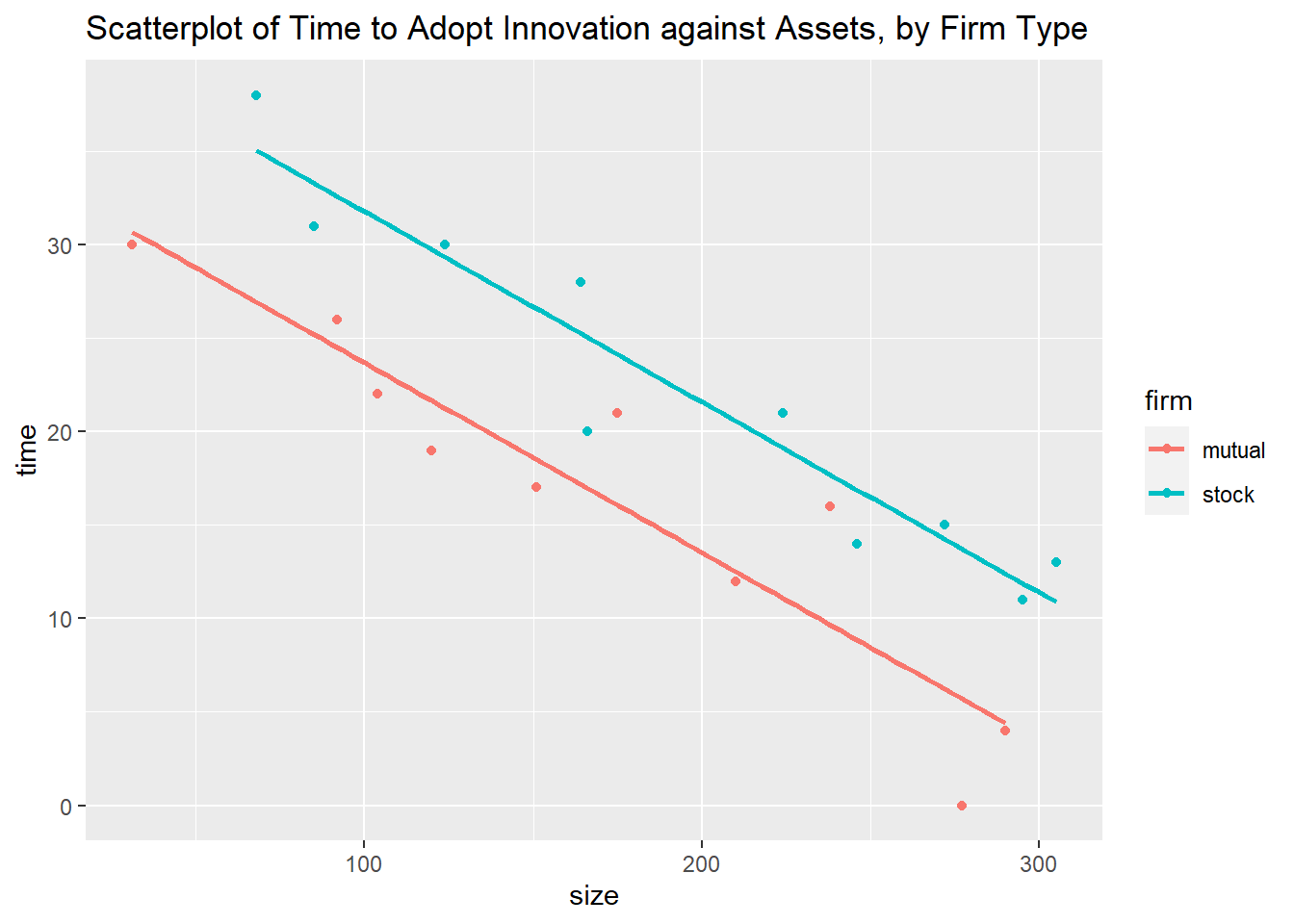

We create a scatterplot of the response variable against the quantitative predictor, with separate colors and lines for firm type. Notice that the lines are almost parallel. We noted earlier that the formulation assumes the slopes are parallel.

\(\beta_1\) denotes the slopes of both of these lines, and \(\beta_2\) denotes how much higher the line is for stock firms than for mutual firms. Let us take a look at the estimated regression coefficients:

result<-lm(time~size+firm, data=Data)
summary(result)

## 
## Call:
## lm(formula = time ~ size + firm, data = Data)
## 
## Residuals:
##     Min      1Q  Median      3Q     Max 
## -5.6915 -1.7036 -0.4385  1.9210  6.3406 
## 
## Coefficients:
##              Estimate Std. Error t value Pr(>|t|)    
## (Intercept) 33.874069   1.813858  18.675 9.15e-13 ***
## size        -0.101742   0.008891 -11.443 2.07e-09 ***
## firmstock    8.055469   1.459106   5.521 3.74e-05 ***
## ---
## Signif. codes:  0 '***' 0.001 '**' 0.01 '*' 0.05 '.' 0.1 ' ' 1
## 
## Residual standard error: 3.221 on 17 degrees of freedom
## Multiple R-squared:  0.8951, Adjusted R-squared:  0.8827 
## F-statistic:  72.5 on 2 and 17 DF,  p-value: 4.765e-09

Note the following from the output:

• We know that since the categorical predictor is binary, we should have only 1 indicator variable representing firm type.

• In the output, note that we have one line for the categorical predictor, called firmstock. This tells us the name of the predictor, followed by the class that is coded 1. So this tells us that R coded stock firms as 1, and mutual firms as 0.

• The estimated coefficient for firmstock is 8.055469. This means that the time to adopt innovation for stock firms is 8.055469 months longer than for mutual firms, when controlling for size of the firm. The associated p-value when testing this coefficient is small, so the data support claim that there is a significant difference in the mean time to adopt inoovation based on firm type, when controlling for size of firm. We do not drop firm type as a term in the model. Since the estimated coefficient is positive, the mean time to adopt innovation for stock firms is longer than for mutual firms, when controlling for size of firm.

• The estimated coefficient for size is -0.101742. This means the time to adopt innovation decreases by 0.101742 months, per unit increase in firm size, for given firm type. The associated p-value when testing this coefficient is small, so we do not drop size as a term in the model.

• The estimated regression equation is \(\hat{y} = 33.874069 - 0.101742 x_1 + 8.055469I_1\).

• Estimated regression equation for mutual firms: \(\hat{y} = 33.874069 - 0.101742 x_1 + 8.055469(0) = 33.874 - 0.102 x_1\).

• Estimated regression equation for stock firms: \(\hat{y} = 33.874069 - 0.101742 x_1 + 8.055469(1) = 41.930 - 0.102 x_1\).

8.2.4 Thought question

How will the output for this regression change if the dummy coding was changed, i.e. \(I_1 = 1\) if mutual firm and 0 if stock firm?

Please view the associated video to review this question, as well as for more commentary on dummy coding.

8.3 Interaction Terms

The regression model as stated in (8.2) is sometimes called a model with additive effects. Additive effects assume that each predictor’s effect on the response does not depend on the value of the other predictor. As long as we hold the other predictor constant, changing the value of the predictor is associated with the same change in the mean response. Using our example, this implies that the when looking at the scatterplot of time to adopt innovation against size of firms, with separate lines for each firm type, the regression lines are parallel.

If the lines are not parallel, it means the effect of changing firm size on the time to adopt innovation depends on the firm type. When the effect of a predictor on the response depends on the value of the other predictor, we have an interaction effect between the predictors on the response variable. To add an interaction effect between the predictors into the model, we have

\[\begin{equation} y = \beta_0 + \beta_1x_{1} + \beta_2I_1 + \beta_3 x_1 I_1 + \epsilon \tag{8.3} \end{equation}\]

where \(I_1 = 1\) if stock firm and 0 if mutual firm. Substituting the values for \(I_1\) in (8.3), we have the following regression equations for each firm type:

• Mutual firm: \(E(y|x) = \beta_0+\beta_2(0)+\beta_1x_1+\beta_3 x_1(0)=\beta_0+\beta_1x_1.\)

• Stock firm: \(E(y|x) = \beta_0+\beta_2(1)+\beta_1x_1+\beta_3 x_1(1)=(\beta_0+\beta_2)+(\beta_1+\beta_3)x_1.\)

We have different intercepts and different slopes for these regressions, whereas in model (8.2), the slopes are the same.

If there is an interaction, we can see the effect of changing \(x_1\) on the response depends on the other predictor: for mutual firms, increasing \(x_1\) by one unit changes the mean response by \(\beta_1\); while for tool stock firms, increasing \(x_1\) by one unit changes the mean response by \(\beta_1 + \beta_3\).

Models with interactions are a bit more difficult to interpret than models with no interactions. Therefore, we typical assess if the interaction term is significant or not. This can be tested in a general linear \(F\) test framework, since a model with additive effects (8.2) is the reduced model and a model with interaction effects (8.3) is the full model. If the coefficient of the interaction term is insignificant, we can drop the interaction term and go with the model with just additive effects.

##model with interaction
result.int<-lm(time~size*firm, data=Data)
summary(result.int) ##can drop interaction

## 
## Call:
## lm(formula = time ~ size * firm, data = Data)
## 
## Residuals:
##     Min      1Q  Median      3Q     Max 
## -5.7144 -1.7064 -0.4557  1.9311  6.3259 
## 
## Coefficients:
##                  Estimate Std. Error t value Pr(>|t|)    
## (Intercept)    33.8383695  2.4406498  13.864 2.47e-10 ***
## size           -0.1015306  0.0130525  -7.779 7.97e-07 ***
## firmstock       8.1312501  3.6540517   2.225   0.0408 *  
## size:firmstock -0.0004171  0.0183312  -0.023   0.9821    
## ---
## Signif. codes:  0 '***' 0.001 '**' 0.01 '*' 0.05 '.' 0.1 ' ' 1
## 
## Residual standard error: 3.32 on 16 degrees of freedom
## Multiple R-squared:  0.8951, Adjusted R-squared:  0.8754 
## F-statistic: 45.49 on 3 and 16 DF,  p-value: 4.675e-08

##can also do general linear F test. same as t test since only dropping one term
anova(result,result.int)

## Analysis of Variance Table
## 
## Model 1: time ~ size + firm
## Model 2: time ~ size * firm
##   Res.Df    RSS Df Sum of Sq     F Pr(>F)
## 1     17 176.39                          
## 2     16 176.38  1 0.0057084 5e-04 0.9821

We look at the result of the \(t\) test for the line size:firmstock, which is the way R denotes the interaction term \(x_1 I_1\). This test is insignificant, we do not have evidence that there is an interaction effect between size of firm and firm type. So we can drop the interaction and go with the simpler model with just additive effects. This is expected given that we have seen almost parallel slopes in the scatterplot.

Note that the hierarchical principle applies if we have an interaction term: if the interaction term is significant, the lower ordered terms must remain.

8.3.1 Consideration of interaction terms

Typically, people start with an additive order model. Interactions considered at the start if:

• Exploring interactions is part of your research question.
• An interaction makes sense contextually, or is well-established in the literature.
• We have evidence of interaction based on visualizations.

8.3.2 Interaction vs correlation

A question that I often get from students have is “Aren’t variables that interact also correlated?” The short answer is no, as interaction and correlation are two very different concepts.

A short explanation is that if we say that there is an interaction between two variables, \(x_1, x_2\), it means how each predictor impacts the response variable \(y\) depends on the value of the other predictor. Notice that there are three variables, \(y, x_1, x_2\) needed when we talk about an interaction between \(x_1, x_2\).

Correlation only involves two variables.

For a more detailed explanation, including examples, please read this page.

8.3.3 Dummy coding vs separate regressions

A reasonable question that is often raised is: Why did we not carry out two separate regressions, one for each firm type? When using dummy coding, we are using one regression. The main reason is that it turns out that using one model with dummy coding leads to more precise estimates (smaller standard errors), than creating separate regression for each level. This is true as long as the regression assumptions are met, specifically that the variance of the errors is constant for both levels.

8.4 Beyond Binary Predictors

If we have a categorical predictor with more than two levels, dummy coding is still used in the same manner: a categorical predictor with \(a\) levels will be represented by \(a-1\) indicator variables, each taking on the values of 0 and 1.

Let us use another example. In this example, we consider ratings of wines from California. The response variable is average quality rating, \(y\), with predictors average flavor rating, \(x_1\), and Region indicating which of three regions in California the wine is produced in. The regions are North, Central, and Napa Valley.

A few notes about using dummy coding in this example:

• Since region has three levels, we will have 2 indicator variables, with one class being the reference class.
• The choice of reference class can be arbitrary, or if there is one class that you are most interested in, make that the reference class.
• The interpretations of the regression model will be consistent regardless of choice for reference class.
• If fitting a model with no interactions, the coefficient of each indicator variable denotes the difference in the mean response between the level that is coded 1 versus the reference class, while controlling for the other predictor.

Let us create a scatterplot of quality rating against flavor rating, split by region:

##clear environment to start new example
rm(list=ls())

Data<-read.table("wine.txt", header=TRUE, sep="")
##convert Region to factor
Data$Region<-factor(Data$Region) 
##assign descriptive labels for each region
levels(Data$Region) <- c("North", "Central", "Napa") 

library(ggplot2)
##scatterplot of Quality against Flavor, 
##separated by Region
ggplot2::ggplot(Data, aes(x=Flavor, y=Quality, color=Region))+
  geom_point()+
  geom_smooth(method=lm, se=FALSE)+
  labs(title="Scatterplot of Wine Quality against Flavor, by Region")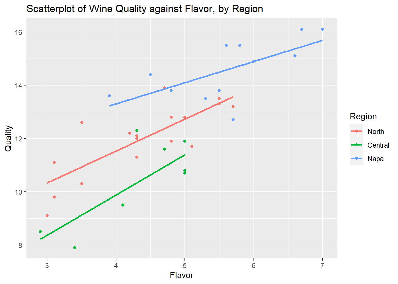

The regression equations are almost parallel so we consider a model with no interactions first. We can use the following indicator variables. Note that there are other ways to define them.

Since Napa Valley is California’s most famous wine region, we would like to make easy comparisons of other regressions with Napa Valley. So it makes sense to make Napa Valley the reference class.

The corresponding model with just additive effects would be

\[\begin{equation*} y_i = \beta_0 + \beta_1x_{i1} + \beta_2I_{i1} + \beta_3I_{i2} + \epsilon_i \end{equation*}\]

So the regression functions are:

• North: \(\mbox{E}\{Y\} = \beta_0 + \beta_1x_1 + \beta_2(1) + \beta_3(0) = (\beta_0+\beta_2) + \beta_1x_1\)

• Central: \(\mbox{E}\{Y\} = \beta_0 + \beta_1x_1 + \beta_2(0) + \beta_3(1) = (\beta_0+\beta_3) + \beta_1x_1\)

• Napa Valley: \(\mbox{E}\{Y\} = \beta_0 + \beta_1x_1 + \beta_2(0) + \beta_3(0) = \beta_0 + \beta_1x_1\)

Recall that this model assumes the slopes are the same for all three regions. \(\beta_{2}\), \(\beta_{3}\) indicate how different the mean ratings are for the North and Central regions compared with Napa Valley, respectively, when controlling for the other predictor, the average flavor rating.

Let us fit this model and look at the output:

##fit regression with no interaction
reduced<-lm(Quality~Flavor+Region, data=Data)
summary(reduced)

## 
## Call:
## lm(formula = Quality ~ Flavor + Region, data = Data)
## 
## Residuals:
##      Min       1Q   Median       3Q      Max 
## -1.97630 -0.58844  0.02184  0.51572  1.94232 
## 
## Coefficients:
##               Estimate Std. Error t value Pr(>|t|)    
## (Intercept)     8.3177     1.0100   8.235 1.31e-09 ***
## Flavor          1.1155     0.1738   6.417 2.49e-07 ***
## RegionNorth    -1.2234     0.4003  -3.056  0.00435 ** 
## RegionCentral  -2.7569     0.4495  -6.134 5.78e-07 ***
## ---
## Signif. codes:  0 '***' 0.001 '**' 0.01 '*' 0.05 '.' 0.1 ' ' 1
## 
## Residual standard error: 0.8946 on 34 degrees of freedom
## Multiple R-squared:  0.8242, Adjusted R-squared:  0.8087 
## F-statistic: 53.13 on 3 and 34 DF,  p-value: 6.358e-13

Some observations from the output:

• \(\hat{\beta_2}\) is the estimated coefficient for the indicator of the North region. This value is -1.2234. We interpret this as the average quality rating for wines in the North region is 1.2234 lower than wines in the Napa Valley, when controlling for flavor rating.

• \(\hat{\beta_3}\) is the estimated coefficient for the indicator of the Central region.The average quality rating for wines in the South region is 2.7569 lower than wines in the Napa Valley, when controlling for flavor rating.

• As mentioned earlier, we can easily make comparisons for any level with the reference class.

8.4.1 Difference in mean response between levels excluding the reference class

Estimating the difference in the mean response between levels excluding the reference class can be done by estimating the difference between the regression coefficients of their respective indicator variables. In this example, \(\beta_2 - \beta_3\) measures the difference in mean response between the North and Central regions, for given average flavor rating. The output from our model does not give us this difference immediately. We can either construct a confidence interval (CI) for \(\beta_2 - \beta_3\), or perform a hypothesis test for \(\beta_2 - \beta_3\).

8.4.1.1 CI

A \(100(1-\alpha)\%\) confidence interval of estimating the differential effects between these regions will be \[\begin{equation} (\hat{\beta}_2-\hat{\beta}_3) \pm t_{1-\alpha/2,n-p}se\left(\hat{\beta}_2-\hat{\beta}_3\right), \tag{8.4} \end{equation}\]

where

\[ Var\left(\hat{\beta}_2-\hat{\beta}_3\right) = Var\left(\hat{\beta}_2\right) + Var\left(\hat{\beta}_3\right) - 2 Cov(\hat{\beta}_2, \hat{\beta}_3). \]

Note that in general, the variance for the difference in estimated coefficients is

\[\begin{equation} Var\left(\hat{\beta}_j-\hat{\beta}_l\right) = Var\left(\hat{\beta}_j\right) + Var\left(\hat{\beta}_l\right) - 2 Cov(\hat{\beta}_j, \hat{\beta}_l). \tag{8.5} \end{equation}\]

We need to obtain the variance-covariance matrix of the estimated coefficients:

##variance covariance matrix of estimated coefficients
round(vcov(reduced),3) ##display 3 dp

##               (Intercept) Flavor RegionNorth RegionCentral
## (Intercept)         1.020 -0.170      -0.277        -0.277
## Flavor             -0.170  0.030       0.037         0.037
## RegionNorth        -0.277  0.037       0.160         0.113
## RegionCentral      -0.277  0.037       0.113         0.202

Let us compute the CI for \(\beta_2 - \beta_3\) using (8.4)

\[\begin{eqnarray*} (\hat{\beta}_2-\hat{\beta}_3) &\pm& t_{1-\alpha/2,n-p}\sqrt{Var\left(\hat{\beta}_2-\hat{\beta}_3\right)} \nonumber \\ (-1.2234 + 2.7569) &\pm& 2.032245 \sqrt{0.160 + 0.202 - 2 \times 0.113} \nonumber \\ (0.7840453&,& 2.2829547) \nonumber \end{eqnarray*}\]

Note \(t_{1-\alpha/2,n-p}\) found using qt(0.975, 38-4).

The CI excludes 0, so there is a significant difference in the mean quality ratings for wines in the North and Central region, when controlling for flavor rating. The CI consists entirely of positive numbers, so the mean quality rating is higher for wines in the North region than the Central region, when controlling for flavor rating.

View the associated video for more in depth explanation for constructing this CI.

8.4.1.2 Hypothesis test

We can also compare between the North and Central regions using hypothesis testing. The hypothesis statements will be:

\[ H_0: \beta_2 - \beta_3 = 0, H_a: \beta_2 - \beta_3 \neq 0. \]

The \(t\) statistic is

\[\begin{eqnarray*} t &=& \frac{\hat{\beta}_2 - \hat{\beta}_3}{se\left(\hat{\beta}_2-\hat{\beta}_3\right)}\nonumber \\ &=& \frac{-1.2234 + 2.7569}{\sqrt{0.160 + 0.202 - 2 \times 0.113}} \nonumber \\ &=& 4.158286, \end{eqnarray*}\]

which is larger than the critical value qt(1-0.05/2, 38 - 4) = 2.032245. So we reject the null hypothesis. Data support the claim that there is a significant difference in the mean quality ratings between wines from the North region and the Central region, when controlling for flavor rating.

8.4.2 Interactions

Suppose we decide to assess if there is an interaction between flavor rating and region. In other words, the effect of flavor rating on quality rating differs by region. From the scatterplot, the slopes are not exactly parallel, so a significant interaction may exist. The model with interaction would be

\[\begin{equation*} y = \beta_0 + \beta_1x_{1} + \beta_2I_{1} + \beta_3I_{2} + \beta_4 x_1 I_{1} + \beta_5 x_1 I_{2} + \epsilon_i \end{equation*}\]

So regression functions are:

• North: \(\mbox{E}\{Y\} = \beta_0 + \beta_1x_1 + \beta_2(1) + \beta_3(0) + \beta_4x_1(1) + \beta_5x_1(0) = (\beta_0+\beta_2) + (\beta_1 + \beta_4)x_1\)

• Central: \(\mbox{E}\{Y\} = \beta_0 + \beta_1x_1 + \beta_2(0) + \beta_3(1) + \beta_4x_1(0) + \beta_5x_1(1) = (\beta_0+\beta_3) + (\beta_1 + \beta_5)x_1\)

• Napa Valley: \(\mbox{E}\{Y\} = \beta_0 + \beta_1x_1 + \beta_2(0) + \beta_3(0) + \beta_4x_1(0) + \beta_5x_1(0) =\beta_0 + \beta_1x_1\)

Let us perform a general linear \(F\) test to see if we should use the model with no interactions or the model with interactions:

##consider model with interactions 
##(when slopes are not parallel)
result<-lm(Quality~Flavor*Region, data=Data)

##general linear F test for interaction terms
anova(reduced,result)

## Analysis of Variance Table
## 
## Model 1: Quality ~ Flavor + Region
## Model 2: Quality ~ Flavor * Region
##   Res.Df    RSS Df Sum of Sq      F Pr(>F)
## 1     34 27.213                           
## 2     32 25.429  2    1.7845 1.1229 0.3378

The general linear \(F\) test is insignificant, so we use the reduced model, i.e. the model with no interactions.

8.5 Pairwise Comparisons

When we have a categorical predictor, we may interested in making comparisons of the mean response between multiple pairs of levels within the categorical predictor. Going back to our wine example, we have a categorical predictor with three levels. This means we can make \(\binom{3}{2} = 3\) pairwise comparisons:

• North region vs Napa Valley
• Central region vs Napa Valley
• North region vs Central region

Based on our indicator variables, the regressions equations

• North: \(\mbox{E}\{Y\} = (\beta_0+\beta_2) + \beta_1x_1\)

• Central: \(\mbox{E}\{Y\} = (\beta_0+\beta_3) + \beta_1x_1\)

• Napa Valley: \(\mbox{E}\{Y\} = \beta_0 + \beta_1x_1\)

So the parameters denoting the pairwise comparisons are

• \(\beta_2\): North region vs Napa Valley
• \(\beta_3\): Central region vs Napa Valley
• \(\beta_2 - \beta_3\): North region vs Central region

To assess whether there is a significant difference in the mean response between each pair, we can either:

1. Conduct 3 hypothesis tests:

   • \(H_0: \beta_2 = 0, H_a: \beta_2 \neq 0\)
   • \(H_0: \beta_3 = 0, H_a: \beta_2 \neq 0\)
   • \(H_0: \beta_3 - \beta_2 = 0, H_a: \beta_3 - \beta_2 \neq 0\)

or

2. Construct 3 confidence intervals:

   • \(\hat{\beta}_2 \pm t_{1- \alpha/2, n-p} se\left( \hat{\beta}_2 \right)\)
   • \(\hat{\beta}_3 \pm t_{1- \alpha/2, n-p} se\left( \hat{\beta}_3 \right)\)
   • \((\hat{\beta}_2 - \hat{\beta}_3) \pm t_{1- \alpha/2, n-p} se\left(\hat{\beta}_2 - \hat{\beta}_3 \right)\)

We have to be careful when conducting multiple tests or constructing multiple CIs.

8.5.1 Significance level

The significance level, \(\alpha\), of a hypothesis test is the probability of wrongly rejecting \(H_0\) if it is true. A Type I error is defined as wrongly rejecting the null hypothesis if it is true. So an alternate definition of the significance level is the probability of making a Type I error, if the null hypothesis is true.

Suppose we conduct the three hypothesis tests to compare all three pairs of regions, each at significance level \(\alpha\). If the null hypothesis is true for all 3 tests (i.e. there is no significant different in mean response between regions, when controlling for flavor), then the probability of making the right conclusions for all of the tests, assuming the tests are independent, will be \((1-\alpha)^3\). If \(\alpha=0.05\), this probability is \(0.95^3 = 0.857375\), not 0.95. A couple of things to consider:

• As we perform more hypothesis tests, the probability of making the right conclusions for all (assuming the null is true for all), decreases.
• Can we do something so that the probability of not making at least one Type I error is still at least \(1-\alpha\)?
• For confidence intervals, we want to ensure that the confidence we have that the entire set of intervals capture the true values of the parameters is still at least \(1-\alpha\).

8.5.2 Multiple pairwise comparisons

To account for the fact that we are making multiple pairwise comparisons, we will need to make our confidence intervals wider, and the critical value larger to ensure the chance of making any Type I error is not more than \(\alpha\). There are a few procedures to do this. We will look two common procedures:

• Bonferroni procedure
• Tukey procedure

With the various procedures in multiple comparison:

1. All the confidence intervals take the form

\[\begin{equation} \text{estimate } \pm \text{ multiplier } \times \text{se(estimate) }. \tag{8.6} \end{equation}\]

2. For hypothesis tests, we reject the null hypothesis when

\[\begin{equation} \text{test statistic } > \text{ critical value}. \tag{8.7} \end{equation}\]

Only the multiplier and critical values change.

8.5.3 Bonferroni procedure

Let \(g\) denote the number of CIs we wish to construct, or the number of hypothesis tests we need to do to perform our pairwise comparisons.

8.5.3.1 CIs

The Bonferroni procedure to ensure that we have at least \((1-\alpha)100\%\) confidence that all the \(g\) CIs capture the true value is

\[\begin{equation} \hat{\beta}_j \pm t_{1-\alpha/(2g); n-p} se(\hat{\beta}_j). \tag{8.8} \end{equation}\]

The multiplier in (8.8) is found using \(t_{1-\alpha/(2g); n-p}\) instead of \(t_{1-\alpha/2; n-p}\).

Going back to the wine example, suppose we wish to make all three pairwise comparisons. The CI to compare the North region with Napa Valley is

\[\begin{eqnarray*} \hat{\beta}_2 &\pm& t_{1-\alpha/(2\times3); 38-4} se(\hat{\beta}_2) \nonumber \\ -1.2234 &\pm& 2.518259 \times 0.4003 \nonumber \\ (-2.2314592 &,& -0.2153408). \nonumber \end{eqnarray*}\]

The CI to compare the Central region with Napa Valley is

\[\begin{eqnarray*} \hat{\beta}_3 &\pm& t_{1-\alpha/(2\times3); 38-4} se(\hat{\beta}_3) \nonumber \\ -2.7569 &\pm& 2.518259 \times 0.4495 \nonumber \\ (-3.888858 &,& -1.624942). \nonumber \end{eqnarray*}\]

The CI to compare the North region with the Central region is

\[\begin{eqnarray*} (\hat{\beta}_2-\hat{\beta}_3) &\pm& t_{1-\alpha/(2\times3); 38-4}\sqrt{Var\left(\hat{\beta}_2-\hat{\beta}_3\right)} \nonumber \\ (-1.2234 + 2.7569) &\pm& 2.518259 \sqrt{0.160 + 0.202 - 2 \times 0.113} \nonumber \\ (0.6048119&,& 2.4621881) \nonumber \end{eqnarray*}\]

All three CIs exclude 0, so there is a significant difference in mean quality rating of wines between all pairs of regions, when controlling for flavor rating.

8.5.3.2 Hypothesis tests

The critical value, based on the Bonferroni procedure, is \(t_{1-\alpha/(2g); n-p}\) (instead of \(t_{1-\alpha/2; n-p}\)). The test statistic still takes the form

\[ t = \frac{\text{estimate}}{s.e. \text{ of estimate}}. \]

To compare the North region with Napa Valley, we have \(H_0: \beta_2 = 0, H_a: \beta_2 \neq 0\). The test statistic is

\[\begin{eqnarray*} t &=& \frac{\hat{\beta}_2}{se(\hat{\beta}_2)} \nonumber \\ &=& \frac{-1.2234}{0.4003} \nonumber \\ &=& -3.056208. \end{eqnarray*}\]

To compare the Central region with Napa Valley, we have \(H_0: \beta_3 = 0, H_a: \beta_3 \neq 0\). The test statistic is

\[\begin{eqnarray*} t &=& \frac{\hat{\beta}_3}{se(\hat{\beta}_3)} \nonumber \\ &=& \frac{-2.7569}{0.4495} \nonumber \\ &=& -6.133259. \end{eqnarray*}\]

To compare the North region with the Central region, we have \(H_0: \beta_2 - \beta_3 = 0, H_a: \beta_2 - \beta_3 \neq 0\). The test statistic is

\[\begin{eqnarray*} t &=& \frac{\hat{\beta}_2 - \hat{\beta}_3}{se(\hat{\beta}_2 - \hat{\beta}_3)} \nonumber \\ &=& \frac{-1.2234 + 2.7569}{\sqrt{0.160 + 0.202 - 2 \times 0.113}} \nonumber \\ &=& 4.158286. \end{eqnarray*}\]

The critical value is 2.518259, found using qt(1-0.05/(2*3), 38-4). The magnitudes of all of these test statistics are larger than the critical value, so there is a significant difference in mean quality rating of wines between which pair of regions, when controlling for flavor rating.

View the associated video and the additional set of notes for an explanation of the rationale behind the Bonferroni procedure.

8.5.4 Tukey procedure

The calculations involved in the Tukey procedure are a little bit more involved so we will not cover the details. We can take a look at some output based on the Tukey procedure:

library(multcomp)
pairwise<-multcomp::glht(reduced, linfct = mcp(Region= "Tukey"))
summary(pairwise)

## 
##   Simultaneous Tests for General Linear Hypotheses
## 
## Multiple Comparisons of Means: Tukey Contrasts
## 
## 
## Fit: lm(formula = Quality ~ Flavor + Region, data = Data)
## 
## Linear Hypotheses:
##                      Estimate Std. Error t value Pr(>|t|)    
## North - Napa == 0     -1.2234     0.4003  -3.056 0.011669 *  
## Central - Napa == 0   -2.7569     0.4495  -6.134  < 1e-04 ***
## Central - North == 0  -1.5335     0.3688  -4.158 0.000606 ***
## ---
## Signif. codes:  0 '***' 0.001 '**' 0.01 '*' 0.05 '.' 0.1 ' ' 1
## (Adjusted p values reported -- single-step method)

Each line is showing the result of testing if the mean quality rating differs between the listed pair of regions (when controlling for flavor rating). We note that the results of all three hypothesis tests are significant. So the data support the claim that there is significant difference in the mean quality of wines between all pairs of regions, when controlling for flavor rating.

Given the negative values for the difference in the estimated coefficients, wines from the Napa valley have the highest ratings, followed by wines from the North region, and then wines from the Central region, when flavor rating is controlled.

8.5.5 Comments about Multiple Comparisons

These procedures to handle multiple pairwise comparisons require there to be no interactions involving the categorical predictor, as we assume the difference in the mean response is the same as long as we control the other predictors.

Some comments about the Bonferroni procedure:

• The probability of making at least one Type I error is \(\leq \alpha\). As \(g\) increases, this probability becomes a lot less than \(\alpha\).
• A by product is that power (the ability to correctly reject the null hypothesis) is sacrificed, especially as \(g\) increases.
• Confidence intervals have a higher level of confidence and are wider.
• Bonferroni procedure is considered conservative (less powerful, wider intervals).
• Fine to use if \(g\) is known prior to looking at the data and is small.
• Easy to implement with simple adjustment to multiplier and critical value.

On the other hand, the Tukey procedure is less conservative and more powerful. Typically used when \(g\) is larger.

8.6 Practical Considerations

8.6.1 Categorical predictor with many levels

For a categorical predictor with many levels, the output can be daunting to look at, as the number of indicator variables (and hence number of regression coefficients) increases as we have more levels. A few things to consider:

• Are you really interested in exploring the differences in the mean response across all the levels?
• Is there a logical way to collapse some levels together that still answers your research question and reduces the number of regression parameters?
• Having more parameters than needed may lead to poorer predictive performance.

8.6.2 Discrete predictors

Do we treat discrete predictors as quantitative or categorical in MLR? A few things to consider:

• Are we fine with assuming they have a ``linear” relationship with the response variable? If yes, more likely we should treat the variable as quantitative.
• How many distinct values are there in the discrete variable? The more distinct values, the more likely we should treat the variable as quantitative.
• Are we concerned about needlessly adding parameters to our model especially if we have a small sample size? If yes, more likely we should treat the variable as quantitative.

8.7 R Tutorial

In this tutorial, we will use the data set wine.txt. The data set contains ratings of various wines produced in California. We will focus on the response variable \(y=\)Quality (average quality rating), \(x_1=\)Flavor (average flavor rating), and Region indicating which of three regions in California the wine is produced in. The regions are coded \(1=\) North, \(2=\) Central, and \(3=\) Napa.

Read the data in and also load the tidyverse package

library(tidyverse)
Data<-read.table("wine.txt", header=TRUE, sep="")
head(Data)

##   Clarity Aroma Body Flavor Oakiness Quality Region
## 1       1   3.3  2.8    3.1      4.1     9.8      1
## 2       1   4.4  4.9    3.5      3.9    12.6      1
## 3       1   3.9  5.3    4.8      4.7    11.9      1
## 4       1   3.9  2.6    3.1      3.6    11.1      1
## 5       1   5.6  5.1    5.5      5.1    13.3      1
## 6       1   4.6  4.7    5.0      4.1    12.8      1

Data Wrangling

Notice from the description that the variable Region is recorded numerically, even though it is a categorical variable. We need to make sure that R is viewing its type correctly by applying the function class() to this variable:

##is Region a factor?
class(Data$Region)

## [1] "integer"

We need to convert Region to be viewed as categorical by using factor(), otherwise R will treat it as a quantitative predictor and not use dummy coding:

##convert Region to factor
Data$Region<-factor(Data$Region) 
##check Region is now the correct type
class(Data$Region) 

## [1] "factor"

We can check how the levels are being described:

##how are levels described
levels(Data$Region)

## [1] "1" "2" "3"

Notice the names of the levels of the regions are not descriptive. We should also give more descriptive names to the levels of Region:

##Give names to the levels
levels(Data$Region) <- c("North", "Central", "Napa") 
levels(Data$Region)

## [1] "North"   "Central" "Napa"

We have done the needed data wrangling: making sure categorical variables are viewed as factors, and giving descriptive names to the levels of the categorical variable.

Note: if categorical variables are already dummy coded, we do not need to convert them to factor when fitting MLR using lm(). The lm() function converts factors to dummy codes.

Scatterplot with categorical predictor

Since we have a quantitative response variable, Quality, a quantitative predictor Flavor and a categorical predictor Region, we can create a scatterplot, with Quality on the y-axis, Flavor on the x-axis, and use different colored plots to denote the different regions:

ggplot2::ggplot(Data, aes(x=Flavor, y=Quality, color=Region))+
  geom_point()+
  geom_smooth(method=lm, se=FALSE)+
  labs(title="Scatterplot of Wine Quality against Flavor, by Region")

We notice a positive linear association between Quality and Flavor across all three regions, the better the flavor of the wine, the higher the quality rating of the wine.

The slopes are not exactly parallel, indicating that there may exist an interaction between the region of the wine and its flavor; the impact of flavor on quality rating differs among the regions. So a regression model with interaction between region and flavor may be appropriate.

Fitting MLR

Since the categorical variable Region has three levels, we know that there will be two indicator variables created to represent the various regions. We check the dummy coding using the contrasts() function:

##check dummy coding
contrasts(Data$Region)

##         Central Napa
## North         0    0
## Central       1    0
## Napa          0    1

This output informs us the North region is the reference class, as it is coded 0 for both indicator variables. We can change the reference class to the Napa region via the relevel() function:

##Set a different reference class
Data$Region<-relevel(Data$Region, ref = "Napa") 
contrasts(Data$Region)

##         North Central
## Napa        0       0
## North       1       0
## Central     0       1

Based on the possibility of non-parallel slopes in the scatterplot, we consider fitting a regression model with an interaction term between the predictors:

result<-lm(Quality~Flavor*Region, data=Data)
summary(result)

## 
## Call:
## lm(formula = Quality ~ Flavor * Region, data = Data)
## 
## Residuals:
##      Min       1Q   Median       3Q      Max 
## -1.94964 -0.58463  0.04393  0.49607  1.97295 
## 
## Coefficients:
##                      Estimate Std. Error t value Pr(>|t|)    
## (Intercept)           10.1144     1.6692   6.060 9.14e-07 ***
## Flavor                 0.7957     0.2936   2.710   0.0107 *  
## RegionNorth           -3.3833     2.0153  -1.679   0.1029    
## RegionCentral         -6.2775     2.4491  -2.563   0.0153 *  
## Flavor:RegionNorth     0.4029     0.3878   1.039   0.3066    
## Flavor:RegionCentral   0.7137     0.4992   1.430   0.1625    
## ---
## Signif. codes:  0 '***' 0.001 '**' 0.01 '*' 0.05 '.' 0.1 ' ' 1
## 
## Residual standard error: 0.8914 on 32 degrees of freedom
## Multiple R-squared:  0.8357, Adjusted R-squared:  0.8101 
## F-statistic: 32.56 on 5 and 32 DF,  p-value: 1.179e-11

##notice hierarchical principle is used

Given that the \(t\) tests for the interaction terms are insignificant, we conduct a partial \(F\) test to see if all the interaction terms can be dropped:

##fit regression with no interaction
reduced<-lm(Quality~Flavor+Region, data=Data)
##general linear F test for interaction terms
anova(reduced,result)

## Analysis of Variance Table
## 
## Model 1: Quality ~ Flavor + Region
## Model 2: Quality ~ Flavor * Region
##   Res.Df    RSS Df Sum of Sq      F Pr(>F)
## 1     34 27.213                           
## 2     32 25.429  2    1.7845 1.1229 0.3378

The insignificant result of the partial \(F\) test means we can drop the interaction terms. There is little evidence that the slopes are truly different.

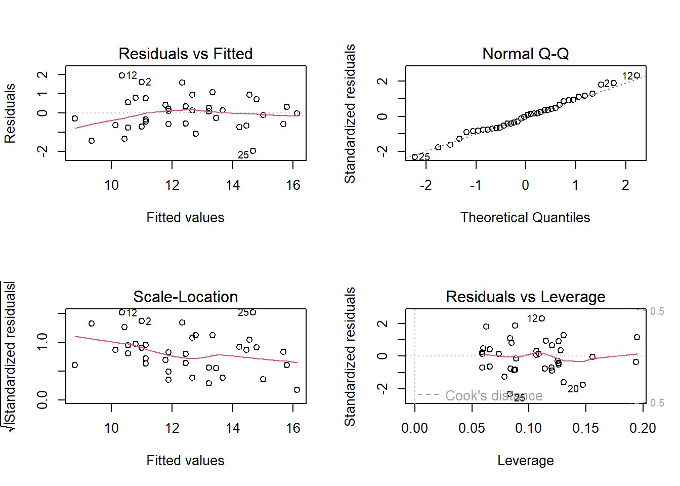
The regression assumptions when a categorical predictor is involved are pretty much the same, assessed similarly as before.

par(mfrow=c(2,2))
plot(reduced)

Multiple comparisons

Since we have a model with no interactions, we can interpret the coefficients of the indicator variables as the difference in the mean quality rating, given the flavor rating, between the class in question and the reference class. Our regression equation is

\[ E(y|x) = \beta_0 + \beta_1 x_1 + \beta_2 I_1 + \beta_3 I_2 \] where \(I_1 = 1\) if North and 0 otherwise, \(I_2 = 1\) if Central and 0 otherwise.

Plugging in the values of the indicator variables, we can write regression equations for each region

• North: \(E(y|x) = \beta_0 + \beta_ 2 + \beta_1 x_1\).
• Central: \(E(y|x) = \beta_0 + \beta_ 3 + \beta_1 x_1\).
• Napa: \(E(y|x) = \beta_0 + \beta_1 x_1\).

Since there are 3 levels, there will be 3 possible pairs of regions to compare (while controlling for flavor rating):

• North and Napa: denoted by \(\beta_ 2\)
• Central and Napa: denoted by \(\beta_ 3\)
• North and Central: \(\beta_2 - \beta_3\)

Let’s take a look at the estimated coefficients

summary(reduced)

## 
## Call:
## lm(formula = Quality ~ Flavor + Region, data = Data)
## 
## Residuals:
##      Min       1Q   Median       3Q      Max 
## -1.97630 -0.58844  0.02184  0.51572  1.94232 
## 
## Coefficients:
##               Estimate Std. Error t value Pr(>|t|)    
## (Intercept)     8.3177     1.0100   8.235 1.31e-09 ***
## Flavor          1.1155     0.1738   6.417 2.49e-07 ***
## RegionNorth    -1.2234     0.4003  -3.056  0.00435 ** 
## RegionCentral  -2.7569     0.4495  -6.134 5.78e-07 ***
## ---
## Signif. codes:  0 '***' 0.001 '**' 0.01 '*' 0.05 '.' 0.1 ' ' 1
## 
## Residual standard error: 0.8946 on 34 degrees of freedom
## Multiple R-squared:  0.8242, Adjusted R-squared:  0.8087 
## F-statistic: 53.13 on 3 and 34 DF,  p-value: 6.358e-13

The estimated difference in the mean quality rating between the sampled wines in the North and Napa regions is -1.22, for given flavor ratings.

The first two comparisons are easy as we can just refer to the coefficients for the indicator variables. A little bit of work needs to be done to compare the North and Central regions. Also, note we are performing three hypothesis tests. So we need to use multiple comparison methods to ensure that the probability of making at least one Type I error is at most the significance level of 0.05.

Bonferroni procedure

As noted earlier, there are 3 pairs of regions to compare (while controlling for flavor rating):

• North and Napa: denoted by \(\beta_ 2\)
• Central and Napa: denoted by \(\beta_ 3\)
• North and `Central: \(\beta_2 - \beta_3\)

The t multiplier and critical value is now \(t_{1-\frac{\alpha}{2g}, n-p}\), which we can find with:

n<-dim(Data)[1]
p<-4
g<-3
t.bon<-qt(1-0.05/(2*g), n-p)
t.bon

## [1] 2.518259

Pairwise comparison with reference class

For the difference in mean quality rating between wines in the North and Napa regions, when controlling for flavor, we use the confidence interval for \(\beta_2\), i.e.,

\[ \hat{\beta}_2 \pm t_{1-\frac{\alpha}{2g}, n-p} se(\hat{\beta}_2) = {-1.2234} \pm 2.518259 \times 0.4003 = (-2.2315, -0.2153) \]

which excludes 0, so we have a significant difference in the mean quality rating between wines in the North and Napa regions, when controlling for flavor. Since the interval is negative, we can say that the mean quality rating for wines in the Napa region is higher than the North region, when controlling for flavor.

To conduct the hypothesis test \(H_0: \beta_2 = 0, H_a: \beta_2 \neq 0\), we can use the critical value (which is the same as the t multiplier) of 2.518259. The test statistic is

\[ \frac{\hat{\beta}_2}{se(\hat{\beta}_2)} = \frac{-1.2234}{0.4003} = -3.056 \] which is larger in magnitude than the critical value, so we reject the null hypothesis.

Notice the result from the confidence interval and hypothesis test are consistent at the same level of significance.

Pairwise comparison excluding reference class

Comparisons excluding the reference require a bit more work. For the difference in mean quality rating between wines in the North and Central regions, when controlling for flavor, we use the CI for \(\beta_2 - \beta_3\):

\[ (\hat{\beta}_2 - \hat{\beta}_3) \pm t_{1-\frac{\alpha}{2g}, n-p} se(\hat{\beta}_2 - \hat{\beta}_3) \]

The output from summary() does not provide \(se(\hat{\beta}_2 - \hat{\beta}_3)\). To obtain the values to calculate this, we need to produce the variance-covariance matrix for the estimated coefficients

vcov(reduced)

##               (Intercept)      Flavor RegionNorth RegionCentral
## (Intercept)     1.0201363 -0.16975148 -0.27722389   -0.27700199
## Flavor         -0.1697515  0.03022282  0.03748222    0.03744271
## RegionNorth    -0.2772239  0.03748222  0.16026554    0.11313506
## RegionCentral  -0.2770020  0.03744271  0.11313506    0.20201780

So we have

\[ Var(\hat{\beta}_2-\hat{\beta}_3) = Var(\hat{\beta}_2) + Var(\hat{\beta}_3) - 2Cov(\hat{\beta}_2,\hat{\beta}_3) = 0.1603 + 0.2020 - 2 \times 0.1131 = 0.1361 \] Therefore, the CI for \(\beta_2 - \beta_3\) is

\[ (-1.2234 - -2.7569 ) \pm 2.518259 \times \sqrt{0.1361} = (0.6045, 2.4625) \] which excludes 0, so we have a significant difference in the mean quality rating between wines in the North and Central regions, when controlling for flavor. Since the interval is positive, we can say that the mean quality rating for wines in the North region is higher than the Central region, when controlling for flavor.

To perform the hypothesis test \(H_0: \beta_2 - \beta_3 = 0, H_a: \beta_2 - \beta_3 \neq 0\), we need to calculate the t-statistic

\[ t-stat = \frac{\hat{\beta}_2 - \hat{\beta}_3}{se(\hat{\beta}_2 - \hat{\beta}_3)} = \frac{-1.2234 - -2.7569}{\sqrt{0.1361}} = 4.1568 \] which is larger in magnitude than the critical value of 2.518259, so we reject the null hypothesis. Again, the conclusions from the hypothesis test and CI are consistent.

Tukey procedure

Another procedure for multiple pairwise comparisons is the Tukey procedure. We use the glht() function from the multcomp package

library(multcomp)
pairwise<-multcomp::glht(reduced, linfct = mcp(Region= "Tukey"))
summary(pairwise)

## 
##   Simultaneous Tests for General Linear Hypotheses
## 
## Multiple Comparisons of Means: Tukey Contrasts
## 
## 
## Fit: lm(formula = Quality ~ Flavor + Region, data = Data)
## 
## Linear Hypotheses:
##                      Estimate Std. Error t value Pr(>|t|)    
## North - Napa == 0     -1.2234     0.4003  -3.056 0.011651 *  
## Central - Napa == 0   -2.7569     0.4495  -6.134  < 1e-04 ***
## Central - North == 0  -1.5335     0.3688  -4.158 0.000573 ***
## ---
## Signif. codes:  0 '***' 0.001 '**' 0.01 '*' 0.05 '.' 0.1 ' ' 1
## (Adjusted p values reported -- single-step method)

We can see that there is a significant difference in the mean Quality rating for all pairs of regions, for given flavor rating, since these tests are all significant.

Given the negative values for the difference in the estimated coefficients, wines from the Napa valley have the highest ratings, followed by wines from the North region, and then wines from the Central region, when flavor rating is controlled.