3 Basics with Simple Linear Regression (SLR)

3.1 Introduction

We will start this module by introducing the simple linear regression model. Simple linear regression uses the term “simple,” because it concerns the study of only one predictor variable with one quantitative response variable. In contrast, multiple linear regression, which we will study in future modules, uses the term “multiple,” because it concerns the study of two or more predictor variables with one quantitative response variable. We start with simple linear regression as it is much easier to visualize concepts in regression models when there is only one predictor variable.

For the time being, we will only consider predictor variables that are quantitative. We will consider predictor variables that are categorical in future modules.

The most common way of visualizing the relationship between one quantitative predictor variable and one quantitative response variable is with a scatter plot. In the simulated example below, we have data from 6000 UVa undergraduate students on the amount of time they spend studying in a week (in minutes), and how many courses they are taking in the semester (3 or 4 credit courses).

##create dataframe
df<-data.frame(study,courses)

##fit regression
result<-lm(study~courses, data=df)

##create scatterplot with regression line overlaid
plot(df$courses, df$study, xlab="# of Courses", ylab="Study Time (Mins)")
abline(result)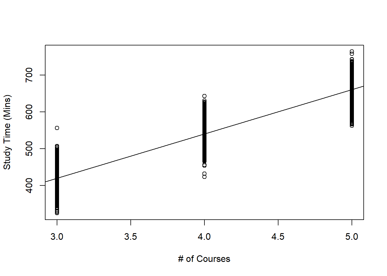

Figure 3.1: Scatterplot of Study Time against Number of Courses Taken

Questions that we may have include:

Are study time and the number of courses taken related to one another?
How strong is this relationship?
Could we use the data to make a prediction for the study time of a student who is not in this scatterplot?
How confident are we of the prediction?

These questions can be answered using simple linear regression.

Note that we will only be learning about models with just one response variable. We will not cover multivariate regression, which is used when there is more than one response variable. There may be some confusion between “multiple” linear regression and “multivariate” regression due to the closeness in terminology.

3.1.1 Basic Ideas with Statistics

3.1.1.1 Population vs Sample

Statistical methods are usually used to make inferences about the population based on information from a sample.

A sample is the collection of units that is actually measured or surveyed in a study.
The population includes all units of interest.

In the study time example above, the population is all UVa undergraduate students, while the sample is the 6000 students that we have data on and are displayed on the scatterplot.

3.1.1.2 Parameters vs Statistics

Parameters are numerical quantities that describe a population.
Statistics are numerical quantities that describe a sample.

In the study time example, an example of a parameter will be the average study time among all UVa undergraduate students (called the population mean), and an example of a statistic will be the average study time among the 6000 UVa students we have data on (called the sample mean).

Notice that in real life, we will rarely know the actual numerical value of a parameter. So we use the numerical value of the statistic to estimate the unknown numerical value of the corresponding parameter.

We also have different notation for parameters and statistics. For example,

the population mean is denoted as $\mu$.
the sample mean is denoted as $\bar{x}$.

We say that $\bar{x}$ is an estimator of $\mu$.

It is important to pay attention to whether we are describing a statistic (a known value that can be calculated) or a parameter (an unknown value).

3.1.2 Motivation

Linear regression models generally have two primary uses:

Prediction: Predict a future value of a response variable, using information from predictor variables.
Association: Quantify the relationship between variables. How does a change in the predictor variable change the value of the response variable?

We always distinguish between a response variable, denoted by $y$, and a predictor variable, denoted by $x$. In most statistical models, we say that the response variable can be approximated by some mathematical function, denoted by $f$, of the predictor variable, i.e.

\[ y \approx f(x). \] Oftentimes, we write this relationship as

\[ y = f(x) + \epsilon, \]

where $\epsilon$ denotes a random error term, with a mean of 0. The error term cannot be predicted based on the data we have.

There are various statistical methods to estimate $f$. Once we estimate $f$, we can use our method for prediction and / or association.

Using the study time example above:

a prediction example: a student intends to take 4 courses in the semester. What is this student’s predicted study time, on average?
an association example: we want to see how taking more courses increases study time.

3.1.2.1 Practice questions

In the examples below, are we using a regression model for prediction or for association?

It is early in the morning and I am heading out for the rest of the day. I want to know the weather forecast for the rest of the day so I know what to wear.
An executive for a sports league wants to assess how increasing the length of commercial breaks may impact the enjoyment of sports fans who watch games on TV.
The Education Secretary would like to evaluate how certain factors such as use of technology in classrooms and investment in teacher training and teacher pay are associated with reading skills of students.
When buying a home, the prospective buyer would like to know if the home is under- or over- priced, given its characteristics.

3.2 Simple Linear Regression (SLR)

In simple linear regression (SLR), the function $f$ that relates the predictor variable with the response variable is typically $\beta_0 + \beta_1 x$. Mathematically, we express this as

\[ y \approx \beta_0 + \beta_1 x, \]

or in other words, that the response variable has an approximately linear relationship with the predictor variable.

In SLR, this relationship is more explicitly formulated as the simple linear regression equation:

\[\begin{equation} E(y|x)=\beta_0+\beta_{1}x. \tag{3.1} \end{equation}\]

$\beta_0$ and $\beta_1$ are parameters in the SLR equation, and we want to estimate them.
These parameters are sometimes called regression coefficients.
$\beta_1$ is also called the slope. It denotes the change in $y$, on average, when $x$ increases by one unit.
$\beta_0$ is also called the intercept. It denotes the average of $y$ when $x=0$.
The notation on the left hand side of (3.1) denotes the expected value of the response variable, for a fixed value of the predictor variable. What (3.1) implies is that, for each value of the predictor variable $x$, the expected value of the response variable $y$ is $\beta_0+\beta_{1}x$. The expected value is also the population mean. Applying (3.1) to our study time example, it implies that:
- for students who take 3 courses, their expected study time is equal to $\beta_0 + 3\beta_1$,
- for students who take 4 courses, their expected study time is equal to $\beta_0 + 4\beta_1$,
- for students who take 5 courses, their expected study time is equal to $\beta_0 + 5\beta_1$.

So $f(x) = \beta_0 + \beta_1x$ gives us the value of the expected value of the response variable for a specific value of the predictor variable. But, for each value of the predictor variable, the value of the response variable is not a constant. We say that for each value of $x$, the response variable $y$ has some variance. The variance of the response variable for each value of $x$ is the same as the variance of the error term, $\epsilon$. Thus we have the simple linear regression model

\[\begin{equation} y=\beta_0+\beta_{1} x + \epsilon. \tag{3.2} \end{equation}\]

We need to make some assumptions for the error term $\epsilon$. Generally, the assumptions are:

The errors have mean 0.
The errors have variance denoted by $\sigma^2$. Notice this variance is constant.
The errors are independent.
The errors are normally distributed.

From (3.2), notice we have another parameter, $\sigma^2$.

We will go into more detail about what these assumptions mean, and how to assess whether they are met, in module 5.

What these assumptions mean is that for each value of the predictor variable $x$, the response variable:

follows a normal distribution,
with mean equal to $\beta_0+\beta_{1} x$,
and variance equal to $\sigma^2$.

Using our study time example, it means that:

for students who take 3 courses, the distribution of their study times is $N(\beta_0 + 3\beta_1, \sigma^2)$.
for students who take 4 courses, the distribution of their study times is $N(\beta_0 + 4\beta_1, \sigma^2)$.
for students who take 5 courses, the distribution of their study times is $N(\beta_0 + 5\beta_1, \sigma^2)$.

So if we were to subset our dataframe into three subsets, one with students who take 3 courses, another subset for students who take 4 courses, and another subset for students who take 5 courses, and then create a density plot of study times for each subset, each density plot should follow a normal distribution, with different means, and the same spread.

Let us take a look at these density plots next.

library(tidyverse)

##subset dataframe
x.3<-df[which(df$courses==3),]
##density plot of study time for students taking 3 courses
ggplot(x.3,aes(x=study))+
  geom_density()+
  labs(x="Study Time (Mins)", title="Dist of Study Times with 3 Courses")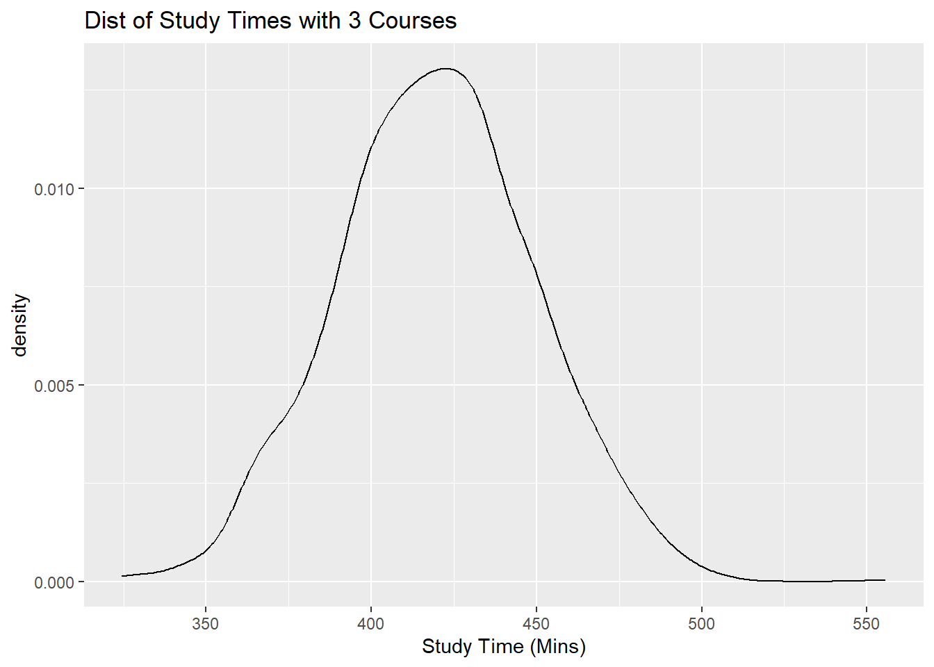

##subset dataframe
x.4<-df[which(df$courses==4),]
##density plot of study time for students taking 4 courses
ggplot(x.4,aes(x=study))+
  geom_density()+
  labs(x="Study Time (Mins)", title="Dist of Study Times with 4 Courses")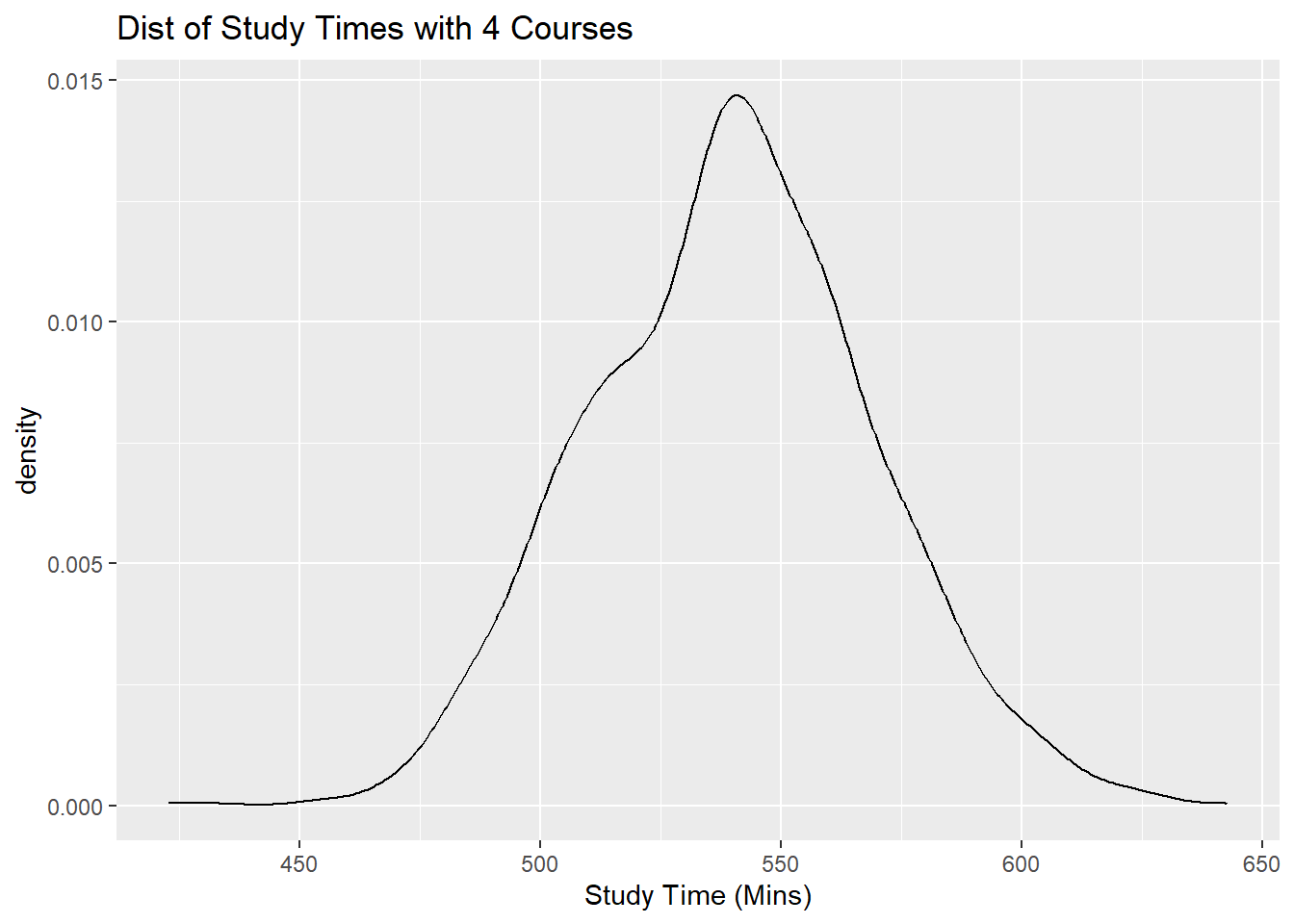

##subset dataframe
x.5<-df[which(df$courses==5),]
##density plot of study time for students taking 5 courses
ggplot(x.5,aes(x=study))+
  geom_density()+
  labs(x="Study Time (Mins)", title="Dist of Study Times with 5 Courses")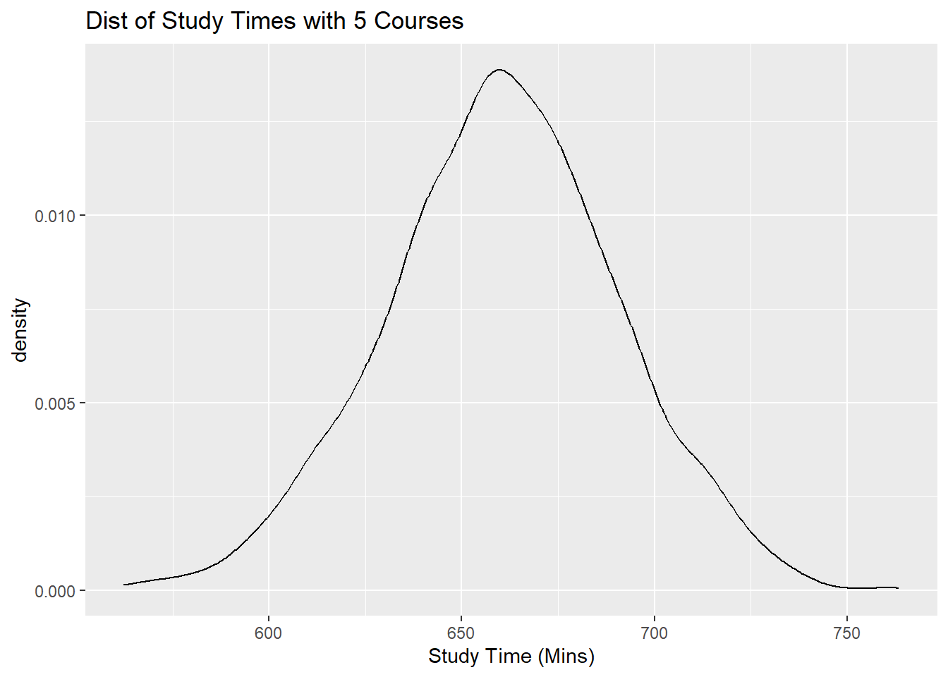

Notice all of these plots are normal, with different means (centers), and similar spreads.

Please see the associated video for more explanation about the distribution of the response variable, for each value of the predictor variable, in an SLR setting.

3.3 Estimating Regression Coefficients in SLR

From (3.1) and (3.2), we noted that we have to estimate the regression coefficients $\beta_0, \beta_1$ as well as the parameter $\sigma^2$ associated with the error term. As mentioned earlier, we are unable to obtain numerical values of these parameters as we do not have data from the entire population. So what we do is use the data from our sample to estimate these parameters.

We estimate $\beta_0,\beta_1$ using $\hat{\beta}_0,\hat{\beta}_1$ based on a sample of observations $(x_i,y_i)$ of size $n$.

The subscripts associated with the response and predictor variables denote which data point that value belongs to. Let us take a look at the first few rows of the data frame for the study time example:

head(df)

##      study courses
## 1 429.8311       3
## 2 458.4588       3
## 3 391.9406       3
## 4 378.0196       3
## 5 397.9856       3
## 6 405.7145       3

For example, $x_1$ denotes the number of courses taken by student number 1 in the dataframe, which is 3. $y_4$ denotes the study time for student number 4 in the dataframe, which is 378.0196456.

Following (3.1) and (3.2), the sample versions are

\[\begin{equation} \hat{y}=\hat{\beta}_0+\hat{\beta}_1 x \tag{3.3} \end{equation}\]

and

\[\begin{equation} y=\hat{\beta}_0+\hat{\beta}_1 x + e \tag{3.4} \end{equation}\]

respectively. (3.3) is called the estimated SLR equation, or fitted SLR equation. (3.4) is called the estimated SLR model.

$\hat{\beta}_1,\hat{\beta}_0$ are the estimators for $\beta_1,\beta_0$ respectively. These estimators can be interpreted in the following manner:

$\hat{\beta}_1$ denotes the change in the predicted $y$ when $x$ increases by 1 unit. Alternatively, it denotes the change in $y$, on average, when $x$ increases by 1 unit.
$\hat{\beta}_0$ denotes the predicted $y$ when $x=0$. Alternatively, it denotes the average of $y$ when $x=0$.

From (3.4), notice we use $e$ to denote the residual, or in other words, the “error” in the sample.

From (3.3) and (3.4), we have the following quantities that we can compute:

\[\begin{equation} \text{Predicted/Fitted values: } \hat{y}_i = \hat{\beta}_0+\hat{\beta}_1 x_i. \tag{3.5} \end{equation}\]

\[\begin{equation} \text{Residuals: } e_i = y_i-\hat{y}_i. \tag{3.6} \end{equation}\]

\[\begin{equation} \text{Sum of Squared Residuals: } SS_{res} = \sum\limits_{i=1}^n(y_i-\hat{y}_i)^2. \tag{3.7} \end{equation}\]

We compute the estimated coefficients $\hat{\beta}_1,\hat{\beta}_0$ using the method of least squares, i.e. choose the numerical values of $\hat{\beta}_1,\hat{\beta}_0$ that minimize $SS_{res}$ as given in (3.7).

By minimizing $SS_{res}$ with respect to $\hat{\beta}_0$ and $\hat{\beta}_1$, the estimated coefficients in the simple linear regression equation are

\[\begin{equation} \hat{\beta}_1 = \frac{\sum\limits_{i=1}^n(x_i-\bar{x})(y_i-\bar{y})}{\sum\limits_{i=1}^n(x_i-\bar{x})^2} \tag{3.8} \end{equation}\]

and

\[\begin{equation} \hat{\beta}_0 = \bar{y}- \hat{\beta}_1 \bar{x} \tag{3.9} \end{equation}\]

$\hat{\beta}_1, \hat{\beta}_0$ are called least squares estimators.

The minimization of $SS_{res}$ with respect to $\hat{\beta}_0$ and $\hat{\beta}_1$ is done by taking the partial derivatives of (3.7) with respect to $\hat{\beta}_1$ and $\hat{\beta}_0$, setting these two partial derivatives equal to 0, and solving these two equations for $\hat{\beta}_1$ and $\hat{\beta}_0$.

Let’s take a look at the estimated coefficients for our study time example:

##fit regression
result<-lm(study~courses, data=df)
##print out the estimated coefficients
result

## 
## Call:
## lm(formula = study ~ courses, data = df)
## 
## Coefficients:
## (Intercept)      courses  
##       58.45       120.39

From our sample of 6000 students, we have

$\hat{\beta}_1$ = 120.3930985. The predicted study time increases by 120.3930985 minutes for each additional course taken.
$\hat{\beta}_0$ = 58.4482853. The predicted study time is 58.4482853 when no courses are taken. Notice this value does not make sense, as a student cannot be taking 0 courses. If you look at our data, the number of courses taken is 3, 4, or 5. So we should only use our regression when $3 \leq x \leq 5$. We cannot use it for values of $x$ outside the range of our data. Making predictions of the response variable for predictors outside the range of the data is called extrapolation and should not be done.

3.4 Estimating Variance of Errors in SLR

The estimator of $\sigma^2$, the variance of the error terms (also the variance of the probability distribution of $y$ given $x$) is \[\begin{equation} s^2 = MS_{res} = \frac{SS_{res}}{n-2} = \frac{\sum\limits_{i=1}^n e_i^2}{n-2}, \tag{3.10} \end{equation}\]

where $MS_{res}$ is the called the mean squared residuals.

$\sigma^2$, the variance of the error terms, measures the spread of the response variable, for each value of $x$. The smaller this is, the closer the data points are to the regression equation.

3.4.1 Practice questions

Take a look at the scatterplot of study time against number of courses taken, Figure 3.1. On this plot, label the following:

estimated SLR equation
the fitted value when $x=3$, $x=4$, and $x=5$.
the residual for any data point on the plot of your choosing.

Try these on your own first, then view the associated video to see if you labeled the plot correctly!

3.5 Assessing Linear Association

As noted earlier, the variance of the error terms inform us how close the data points are to the estimated SLR equation. The smaller the variance of the error terms, the closer the data points are to the estimated SLR equation. This in turn implies the linear relationship between the variables is stronger.

We will learn about some common measures that are used to quantify the strength of the linear relationship between the response and predictor variables. Before we do that, we need to define some other terms.

3.5.1 Sum of squares

\[\begin{equation} \text{Total Sum of Squares: } SS_T = \sum\limits_{i=1}^{n} (y_i - \bar{y})^{2}. \tag{3.11} \end{equation}\]

Total sum of squares is defined as the total variance in the response variable. The larger this value is, the larger the spread is of the response variable.

\[\begin{equation} \text{Regression sum of squares: } SS_R = \sum\limits_{i=1}^{n} (\hat{y_i} - \bar{y})^{2}. \tag{3.12} \end{equation}\]

Regression sum of squares is defined as the variance in the response variable that can be explained by our regression.

We also have residual sum of squares, $SS_{res}$. Its mathematical formulation is given in (3.7). It is defined as the variance in the response variable that cannot be explained by our regression.

It can be shown that

\[\begin{equation} SS_T = SS_R + SS_{res}. \tag{3.13} \end{equation}\]

Each of the sums of squares has its associated degrees of freedom (df):

df for $SS_R$: $df_R = 1$
df for $SS_{res}$: $df_{res} = n-2$
df for $SS_T$: $df_T = n-1$

Please see the associated video for more explanation about the concept behind degrees of freedom.

3.5.2 ANOVA Table

Information regarding the sums of squares is usually presented in the form of an ANOVA (analysis of variance) table:

Source of Variation	SS	df	MS	F
Regression	$SS_R=\sum\left(\hat{y_i}-\bar{y}\right)^2$	$df_R = 1$	$MS_R=\frac{SS_R}{df_R}$	$\frac{MS_R}{MS_{res}}$
Error	$SS_{res} = \sum\left(y_i-\hat{y_i}\right)^2$	$df_{res} = n-2$	$MS_{res}=\frac{SS_{res}}{df_{res}}$	`***`
Total	$SS_T=\sum\left(y_i-\bar{y}\right)^2$	$df_T = n-1$	`***`	`***`

Note:

Dividing each sum of square with its corresponding degrees of freedom gives the corresponding mean square.
In the last column, we report an $F$ statistic, which equal to $\frac{MS_R}{MS_{res}}$. This $F$ statistic is associated with an ANOVA F test, which we will look at in more detail in the next subsection.

To obtain the ANOVA table for our study time example:

anova(result)

## Analysis of Variance Table
## 
## Response: study
##             Df   Sum Sq  Mean Sq F value    Pr(>F)    
## courses      1 57977993 57977993   65404 < 2.2e-16 ***
## Residuals 5998  5317017      886                      
## ---
## Signif. codes:  0 '***' 0.001 '**' 0.01 '*' 0.05 '.' 0.1 ' ' 1

Notice that R does not print out the information for the line regarding $SS_T$.

3.5.3 ANOVA $F$ Test

In SLR, the ANOVA $F$ statistic from the ANOVA table can be used to test if the slope of the SLR equation is 0 or not. In words, this means that whether there is a linear association between the variables or not. If the slope is 0, it means that changes in the value of the predictor variable do not change the value of the response variable, on average; hence the variables are not linearly associated.

The null and alternative hypotheses are:

\[ H_0: \beta_1 = 0, H_a: \beta_1 \neq 0. \] The test statistic is

\[\begin{equation} F = \frac{MS_R}{MS_{res}} \tag{3.14} \end{equation}\]

and is compared with an $F_{1,n-2}$ distribution. Note that $F_{1,n-2}$ is read as an F distribution with 1 and $n-2$ degrees of freedom.

Going back to the study time example, the $F$ statistic is 6.5403586^{4}. The critical value can be found using

qf(1-0.05, 1, 6000-2)

## [1] 3.84301

Since our test statistic is larger than the critical value, we reject the null hypothesis. Our data support the claim that the slope is different from 0, or in other words, that there is a linear association between study time and number of courses taken.

3.5.4 Coefficient of determination

The coefficient of determination, $R^2$, is

\[\begin{equation} R^{2} = \frac{SS_R}{SS_T} = 1 - \frac{SS_{res}}{SS_T}. \tag{3.15} \end{equation}\]

$R^{2}$ is an indication of how well the data fits our model. In the context of simple linear regression, it denotes the proportion of variance in the response variable that is explained by the predictor.

A few notes about $R^2$:

$0 \leq R^2 \leq 1$.
Values closer to 1 indicate a better fit; values closer to 0 indicate a poorer fit.
Sometimes reported as a percentage.

To obtain $R^2$ for our study time example:

anova.tab<-anova(result)
##SST not provided, so we add up SSR and SSres
SST<-sum(anova.tab$"Sum Sq")
##R2
anova.tab$"Sum Sq"[1]/SST

## [1] 0.9159963

This implies that the proportion of variance in study time that can be explained by the number of courses taken is 0.9159963.

3.5.5 Correlation

A measure used to quantify the strength of the linear association between two quantitative variables is the sample correlation. The sample correlation, $\mbox{Corr}(x,y)$ or $r$, is given by

\[\begin{equation} r = \frac{\sum\limits_{i=1}^{n}(x_i - \bar{x})(y_i - \bar{y})}{\sqrt{\sum\limits_{i=1}^{n}(x_i - \bar{x})^{2}(y_i - \bar{y})^{2}}}. \tag{3.16} \end{equation}\]

A few notes about $r$:

$-1 \leq r \leq 1$.
Sign of correlation indicates direction of association. A positive value indicates a positive linear association: as the predictor variable increases, so does the response variable, on average. A negative value indicates a negative linear association: as the predictor variable increases, the response variable decreases, on average.
Values closer to 1 or -1 indicate a stronger linear association; values closer to 0 indicate a weaker linear association.
In SLR, it turns out that $r^2 = R^2$.

Using our study time example, the correlation between study time and number of courses taken is

cor(df$study, df$courses)

## [1] 0.9570769

This value indicates a very strong and positive linear association between study time and number of courses taken (remember that this is simulated data and is not real).

3.5.5.1 How strong is strong?

A question that is often raised is how large should the magnitude of the sample correlation be for it to be considered strong? The answer is: it depends on the context. If you are conducting an experiment that is governed by scientific laws (e.g an experiment verifying Newton’s 2nd law that $F = ma$), we should expect an extremely high correlation. A correlation of 0.9 in such an instance may be considered weak. The value of the correlation you have should be compared with correlations from similar studies in that domain to determine if it is strong or not.

3.6 A Word of Caution

To be able to use the measures we have learned (such as correlation, $R^2$) and to interpret the estimated regression coefficients, we must verify via a scatterplot that the association between the two variables is approximately linear. If we see a non linear pattern in the scatterplot, we should not use or interpret these values. We will learn how to remedy the situation if we see a non linear pattern in the scatterplot in module 5.

Please see the associated video for a demonstration on how not looking at the scatterplot can lead to misleading interpretations.

3.7 R Tutorial

For this tutorial, we will work with the dataset elmhurst from the openintro package in R.

library(tidyverse)
library(openintro)
Data<-openintro::elmhurst

Type ?openintro::elmhurst to read the documentation for datasets in R. Always seek to understand the background of your data! The key pieces of information are:

A random sample of 50 students (all freshman from the 2011 class at Elmhurst College).
Family income of the student (units are missing).
Gift aid, in $1000s.

We want to explore how family income may be related to gift aid, in a simple linear regression framework.

Visualization

We should always verify with scatterplot that the relationship is (approximately) linear before proceeding with correlation and simple linear regression!

##scatterplot of gift aid against family income
ggplot2::ggplot(Data, aes(x=family_income,y=gift_aid))+
  geom_point()+
  geom_smooth(method = "lm", se=FALSE)+
  labs(x="Family Income", y="Gift Aid", title="Scatterplot of Gift Aid against Family")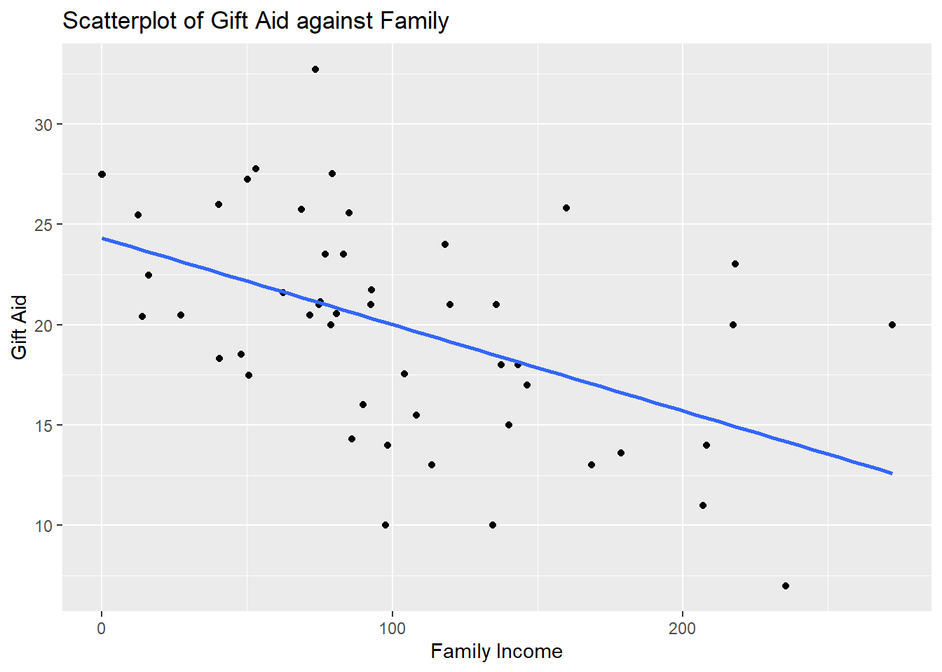

We note that the observations are fairly evenly scattered on both sides of the regression line, so a linear association exists. We see a negative linear association. As family income increases, the gift aid, on average, decreases.

We also do not see any observation with weird values that may warrant further investigation.

Regression

We use the lm() function to fit a regression model:

##regress gift aid against family income
result<-lm(gift_aid~family_income, data=Data)

Use the summary() function to display relevant information from this regression:

##look at information regarding regression
summary(result)

## 
## Call:
## lm(formula = gift_aid ~ family_income, data = Data)
## 
## Residuals:
##      Min       1Q   Median       3Q      Max 
## -10.1128  -3.6234  -0.2161   3.1587  11.5707 
## 
## Coefficients:
##               Estimate Std. Error t value Pr(>|t|)    
## (Intercept)   24.31933    1.29145  18.831  < 2e-16 ***
## family_income -0.04307    0.01081  -3.985 0.000229 ***
## ---
## Signif. codes:  0 '***' 0.001 '**' 0.01 '*' 0.05 '.' 0.1 ' ' 1
## 
## Residual standard error: 4.783 on 48 degrees of freedom
## Multiple R-squared:  0.2486, Adjusted R-squared:  0.2329 
## F-statistic: 15.88 on 1 and 48 DF,  p-value: 0.0002289

We see the following values:

$\hat{\beta}_1 =$ -0.0430717. The estimated slope informs us the the predicted gift aid decreases by 0.0430717 thousands of dollars (or $43.07) per unit increase in family income.
$\hat{\beta}_0 =$ 24.319329. For students with no family income, their predicted gift aid is $24 319.33. Note: from the scatterplot, we have an observation with 0 family income. We must be careful in not extrapolating when making predictions with our regression. We should only make predictions for family incomes between the minimum and maximum values of family incomes in our data.
$s$ = 4.7825989, is the estimate of the standard deviation of the error terms. This is reported as residual standard error in R. Squaring this gives the estimated variance.
$F$ = 15.8772043. This is the value of the ANOVA $F$ statistic. The corresponding p-value is reported. Since this p-value is very small, we reject the null hypothesis. The data support the claim that there is a linear association between gift aid and family income.
$R^2 =$ 0.2485582. The coefficient of determination informs us that about 24.86% of the variation in gift aid can be explained by family income.

Extract values from R objects

We can actually extract these values that are being reported from summary(result). To see what can be extracted from an R object, use the names() function:

##see what can be extracted from summary(result)
names(summary(result))

##  [1] "call"          "terms"         "residuals"     "coefficients" 
##  [5] "aliased"       "sigma"         "df"            "r.squared"    
##  [9] "adj.r.squared" "fstatistic"    "cov.unscaled"

To extract the estimated coefficients:

##extract coefficients
summary(result)$coefficients

##                  Estimate Std. Error   t value     Pr(>|t|)
## (Intercept)   24.31932901 1.29145027 18.831022 8.281020e-24
## family_income -0.04307165 0.01080947 -3.984621 2.288734e-04

Notice the information is presented in a table. To extract a specific value, we can specify the row and column indices:

##extract slope
summary(result)$coefficients[2,1]

## [1] -0.04307165

##extract intercept
summary(result)$coefficients[1,1]

## [1] 24.31933

On your own, extract the values of the residual standard error, the ANOVA F statistic, and $R^2$.

Prediction

A use of regression models is prediction. Suppose I want to predict the gift aid of a student with family income of 50 thousand dollars (assuming the unit is in thousands of dollars). We use the predict() function:

##create data point for prediction
newdata<-data.frame(family_income=50)
##predicted gift aid when x=50
predict(result,newdata)

##        1 
## 22.16575

This student’s predicted gift aid is $22 165.75. Alternatively, you could have calculated this by plugging $x=50$ into the estimated SLR equation:

summary(result)$coefficients[1,1] + summary(result)$coefficients[2,1]*50

## [1] 22.16575

ANOVA table

We use the anova() function to display the ANOVA table

anova.tab<-anova(result)
anova.tab

## Analysis of Variance Table
## 
## Response: gift_aid
##               Df  Sum Sq Mean Sq F value    Pr(>F)    
## family_income  1  363.16  363.16  15.877 0.0002289 ***
## Residuals     48 1097.92   22.87                      
## ---
## Signif. codes:  0 '***' 0.001 '**' 0.01 '*' 0.05 '.' 0.1 ' ' 1

The report $F$ statistic is the same as the value reported earlier from summary(result).

The first line of the output gives $SS_{R}$, the second line gives $SS_{res}$. The function doesn’t provide $SS_T$, but we know that $SS_T = SS_{R} + SS_{res}$.

Again, to see what can be extracted from anova.tab:

names(anova.tab)

## [1] "Df"      "Sum Sq"  "Mean Sq" "F value" "Pr(>F)"

So $SS_T$ can be easily calculated:

SST<-sum(anova.tab$"Sum Sq")
SST

## [1] 1461.079

The $R^2$ was reported to be 0.2485582. To verify using the ANOVA table:

anova.tab$"Sum Sq"[1]/SST

## [1] 0.2485582

Correlation

We use the cor() function to find the correlation between two quantitative variables:

##correlation
cor(Data$family_income,Data$gift_aid)

## [1] -0.4985561

The correlation is -0.4985561. We have a moderate, negative linear association between family income and gift aid.

2 Data Visualization with R Using ggplot2

4 Inference with Simple Linear Regression (SLR)

Linear Models for Data Science