4 Inference with Simple Linear Regression (SLR)

4.1 Introduction

Oftentimes, the data we collect come from a random sample that is representative of the population of interest. A common example is an election poll before a presidential election. Random sampling allows the sample to be representative of the population. However, if we obtain another random sample, the characteristics of the new sample are unlikely to be exactly the same as the first sample. For example, the sample proportion who will vote for a certain party is unlikely to be the same for both random samples. What this tells us is that even with representative samples, sample proportions are unlikely to be equal to the population proportion, and sample proportions vary from sample to sample.

Dr. W. Edwards Deming’s Red Bead experiment illustrates this concept. A video of this experiment can be found here.

In this video, the number of red beads, which represent bad products, varies each time the worker obtains a random sample of 50 beads. The fact that the number of red beads increases in his second sample does not indicate that he performed his task any worse, as this increase is due to the random variation associated with samples.

Note: Deming’s Red Bead experiment was developed to illustrate concepts associated with management. He is best known for his work in developing the Japanese economy after World War II. You will be able to find many blogs/articles discussing the experiment on the World Wide Web. Although many of the articles discuss how this experiment applies in management, it can be used to illustrate concepts of variation.

The same idea extends to the slope and intercept of a regression line. The estimated slope and intercept will vary from sample to sample and are unlikely to be equal to the population slope and intercept. In inferential statistics, we use hypothesis tests and confidence intervals to aid us in accounting for this random variation. In this module, you will learn how to account for and quantify the random variation associated with the estimated regression model, and how to interpret the estimated regression model while accounting for random variation.

4.1.1 Review from previous module

The simple linear regression model is written as

\[\begin{equation} y=\beta_0+\beta_{1} x + \epsilon. \tag{4.1} \end{equation}\]

We make some assumptions for the error term $\epsilon$. They are:

The errors have mean 0.
The errors have variance denoted by $\sigma^2$. Notice this variance is constant.
The errors are independent.
The errors are normally distributed.

These assumptions allow us to derive the distributional properties associated with our least squares estimators $\hat{\beta}_0, \hat{\beta}_1$, which then enables us to compute reliable confidence intervals and perform hypothesis tests on our SLR reliably.

$\hat{\beta}_1,\hat{\beta}_0$ are the estimators for $\beta_1,\beta_0$ respectively. These estimators can be interpreted in the following manner:

$\hat{\beta}_1$ denotes the change in the predicted $y$ when $x$ increases by 1 unit. Alternatively, it denotes the change in $y$, on average, when $x$ increases by 1 unit.
$\hat{\beta}_0$ denotes the predicted $y$ when $x=0$. Alternatively, it denotes the average of $y$ when $x=0$.

How do the values of these estimators vary from sample to sample?

4.2 Hypothesis Testing in SLR

4.2.1 Distribution of least squares estimators

Gauss Markov Theorem: Under assumptions for a regression model, the least squares estimators $\hat{\beta}_1$ and $\hat{\beta}_0$ are unbiased and have minimum variance among all unbiased linear estimators.

Thus, the least squares estimators have the following properties:

$\mbox{E}(\hat{\beta}_1) = \beta_1$, $\mbox{E}(\hat{\beta}_0) = \beta_0$

Note: An estimator is unbiased if its expected value is exactly equal to the parameter it is estimating.

The variance of $\hat{\beta}_1$ is

\[\begin{equation} \mbox{Var}(\hat{\beta}_1) = \frac{\sigma^{2}}{\sum{(x_{i}-\bar{x})^{2}}} \tag{4.2} \end{equation}\]

The variance of $\hat{\beta}_0$ is

\[\begin{equation} \mbox{Var}(\hat{\beta}_0) = \sigma^2 \left[\frac{1}{n} + \frac{\bar{x}^2}{\sum (x_i -\bar{x})^2}\right] \tag{4.3} \end{equation}\]

$\hat{\beta}_1$ and $\hat{\beta}_0$ both follow a normal distribution.

Note that in (4.2) and (4.3), we use $s^2 = MS_{res}$ to estimate $\sigma^2$ since $\sigma^2$ is a unknown value.

What these imply is that if we standardize $\hat{\beta}_1$ and $\hat{\beta}_0$, these standardized quantities will follow a $t_{n-2}$ distribution, i.e.

\[\begin{equation} \frac{\hat{\beta}_1 - \beta_1}{se(\hat{\beta}_1)}\sim t_{n-2} \tag{4.4} \end{equation}\]

and

\[\begin{equation} \frac{\hat{\beta}_0 - \beta_0}{se(\hat{\beta}_0)}\sim t_{n-2}, \tag{4.5} \end{equation}\]

where

\[\begin{equation} se(\hat{\beta}_1) = \sqrt{\frac{MS_{res}}{\sum{(x_{i}-\bar{x})^{2}}}} = \frac{s}{\sqrt{\sum{(x_{i}-\bar{x})^{2}}}} \tag{4.6} \end{equation}\]

and

\[\begin{equation} se(\hat{\beta}_0) = \sqrt{MS_{res}\left[\frac{1}{n} + \frac{\bar{x}^2}{\sum (x_i -\bar{x})^2}\right]} = s \sqrt{\frac{1}{n} + \frac{\bar{x}^2}{\sum (x_i -\bar{x})^2}} \tag{4.7} \end{equation}\]

Note:

$se(\hat{\beta}_1)$ is read as the standard error of $\hat{\beta}_1$. The standard error of any estimator is essentially the sample standard deviation of that estimator, and measures the spread of that estimator.
A $t_{n-2}$ distribution is read as a $t$ distribution with $n-2$ degrees of freedom.

4.2.2 Testing regression coefficients

Hypothesis testing is used to investigate if a population parameter is different from a specific value. In the context of SLR, we usually want to test if $\beta_1$ is 0 or not. If $\beta_1 = 0$, there is no linear relationship between the variables.

The general steps in hypothesis testing are:

Step 1: State the null and alternative hypotheses.
Step 2: A test statistic is calculated using the sample, assuming the null is true. The value of the test statistic measures how the sample deviates from the null.
Step 3: Make conclusion, using either critical values or p-values.

In the previous module, we introduced the ANOVA $F$ test. In SLR, this tests if the slope of the SLR equation is 0 or not. It turns out that we can also perform a $t$ test for the slope. In the $t$ test for the slope, the null and alternative hypotheses are:

\[ H_0: \beta_1 = 0, H_a: \beta_1 \neq 0. \] The test statistic is

\[\begin{equation} t = \frac{\hat{\beta}_1 - \text{ value in null}}{se(\hat{\beta}_1)} \tag{4.8} \end{equation}\]

which is compared with a $t_{n-2}$ distribution. Notice that (4.8) comes from (4.4).

Let us go back to our simulated example that we saw in the last module. We have data from 6000 UVa undergraduate students on the amount of time they spend studying in a week (in minutes), and how many courses they are taking in the semester (3 or 4 credit courses).

##create dataframe
df<-data.frame(study,courses)

##fit regression
result<-lm(study~courses, data=df)
##look at regression coefficients
summary(result)$coefficients

##              Estimate Std. Error   t value      Pr(>|t|)
## (Intercept)  58.44829  1.9218752  30.41211 4.652442e-189
## courses     120.39310  0.4707614 255.74125  0.000000e+00

The $t$ statistic for testing $H_0: \beta_1 = 0, H_a: \beta_1 \neq 0$ is reported to be 255.7412482, which can be calculated using (4.8): $t= \frac{120.39310 - 0}{0.4707614}$. The reported p-value is virtually 0, so we reject the null hypothesis. The data support the claim that there is a linear association between study time and the number of courses taken.

4.3 Confidence Intervals for Regression Coefficients

Confidence intervals (CIs) are similar to hypothesis testing in the sense that they are also based on the distributional properties of an estimator. CIs may differ in their use in the following ways:

We are not assessing if the parameter is different from a specific value.
We are more interested in exploring a plausible range of values for an unknown parameter.

Because CIs and hypothesis tests are based on the distributional properties of an estimator, their conclusions will be consistent (as long as the significance level is the same).

Recall the general form for CIs:

\[\begin{equation} \mbox{estimator} \pm (\mbox{multiplier} \times \mbox{s.e of estimator}). \tag{4.9} \end{equation}\]

We have the following components of a CI

estimator (or statistic): numerical quantity that describes a sample
multiplier: determined by confidence level and relevant probability distribution
standard error of estimator: measure of variance of estimator (basically the square root of the variance of estimator)

Following (4.9) and (4.4), the $100(1-\alpha)\%$ CI for $\beta_1$ is

\[\begin{equation} \hat{\beta}_1 \pm t_{1-\alpha/2;n-2} se(\hat{\beta}_1) = \hat{\beta}_1 \pm t_{1-\alpha/2;n-2} \frac{s}{\sqrt{\sum(x_i - \bar{x})^{2}}}. \tag{4.10} \end{equation}\]

Going back to our study time example, the 95% CI for $\beta_1$ is (119.470237, 121.3159601).

##CI for coefficients
confint(result,level = 0.95)[2,]

##    2.5 %   97.5 % 
## 119.4702 121.3160

An interpretation of this CI is that we have 95% confidence that the true slope $\beta_1$ lies between (119.470237, 121.3159601). In other words, for each additional course taken, the predicted study time increases between 119.470237 and 121.3159601 minutes.

4.3.1 Thought questions

Is the conclusion from this 95% CI consistent with the hypothesis test for $H_0: \beta_1 = 0$ in the previous section at 0.05 significance level?
I have presented hypothesis tests and CIs for the slope, $\beta_1$.
- How would you calculate the $t$ statistic if you wanted to test $H_0: \beta_0 = 0, H_0: \beta_0 \neq 0$?
- How would you calculate the 95% CI for the intercept $\beta_0$?

Generally, we are usually more interested in the slope than the intercept.

4.4 CI of the Mean Response

We have established that the least squares estimators $\hat{\beta}_1,\hat{\beta}_0$ have their associated variances. Since the estimated SLR equation is

\[\begin{equation} \hat{y}=\hat{\beta}_0+\hat{\beta}_1 x, \tag{4.11} \end{equation}\]

it stands to reason that $\hat{y}$ has an associated variance as well, since it is a function of $\hat{\beta}_1,\hat{\beta}_0$.

There are two interpretations of $\hat{y}$:

it estimates the mean of $y$ when $x=x_0$;
it predicts the value of $y$ for a new observation when $x=x_0$.

Note: $x_0$ denotes a specific numerical value for the predictor variable.

Depending on which interpretation we want, there are two different intervals based on $\hat{y}$. The first interpretation is associated with the confidence interval for the mean response, $\hat{\mu}_{y|x_0}$, given the predictor. This is used when we are interested in the average value of the response variable, when the predictor is equal to a specific value. This CI is

\[\begin{equation} \hat{\mu}_{y|x_0}\pm t_{1-\alpha/2,n-2}s\sqrt{\frac{1}{n} + \frac{(x_0-\bar{x})^2}{\sum(x_i-\bar{x})^2}}. \tag{4.12} \end{equation}\]

Going back to our study time example, suppose we want the average study time for students who take 5 courses, the 95% CI is

##CI for mean y when x=5
newdata<-data.frame(courses=5)
predict(result, newdata, level=0.95, interval="confidence")

##        fit      lwr      upr
## 1 660.4138 659.2224 661.6052

We have 95% confidence that the average study time for students who take 5 courses is between 659.2223688 and 661.605187 minutes.

4.5 PI of a New Response

Previously, we found a CI for the mean of $y$ given a specific value of $x$, (4.12). This CI gives us an idea about the location of the regression line at a specific of $x$.

Instead, we may have interest in finding an interval for a new value of $\hat{y}_0$, when we have a new observation $x=x_0$. This is called a prediction interval (PI) for a future observation $y_0$ when the predictor is a specific value. This interval follows from the second interpretation of $\hat{y}$.

The PI for $\hat{y}_0$ takes into account:

Variation in location for the distribution of $y$ (i.e. where is the center of the distribution of $y$?).
Variation within the probability distribution of $y$.

By comparison, the confidence interval for the mean response (4.12) only takes into account the first element. The PI is

\[\begin{equation} \hat{y}_0\pm t_{1-\alpha/2,n-2}s \sqrt{1+\frac{1}{n} + \frac{(x_0-\bar{x})^2}{\sum(x_i-\bar{x})^2}}. \tag{4.13} \end{equation}\]

Going back to our study time example, suppose we have a newly enrolled student who wishes to take 5 courses, and the student wants to predict his study time

##PI for y when x=5
predict(result, newdata, level=0.95, interval="prediction")

##        fit      lwr      upr
## 1 660.4138 602.0347 718.7928

We have 95% confidence that the study time for this student is between 602.0347305 and 718.7928253 minutes.

4.5.1 Thought questions

In the following two scenarios, decide if we are more interested in the CI for the mean response given the predictor (4.12), or the PI for a future response given the predictor (4.13).
- We wish to estimate the waiting time, on average, of DMV customers if there are 10 people in line at the DMV.
- I enter the DMV and notice 10 people in line. I want to estimate my waiting time.
Look at the standard errors associated with the intervals given in (4.12) and (4.13). How are they related to each other?

4.6 Supplemental Notes on Statistical Inference

4.6.1 Hypothesis statements

Let’s consider a $t$ test for the regression parameter, $\beta_1$. Depending on context, the following could be null and alternative hypotheses

$H_0: \beta_1 = 0, H_a: \beta_1 \neq 0$.
$H_0: \beta_1 = 0, H_a: \beta_1 > 0$.
$H_0: \beta_1 = 0, H_a: \beta_1 < 0$.

The null hypothesis should be stated as a statement of equality. This concept holds true for hypothesis tests in general. Some other books / resources might state them as

$H_0: \beta_1 = 0, H_a: \beta_1 \neq 0$.
$H_0: \beta_1 \leq 0, H_a: \beta_1 > 0$.
$H_0: \beta_1 \geq 0, H_a: \beta_1 < 0$.

I prefer using the equality statement for the null hypothesis for the following reasons (theoretical, pedagogical, practical):

The null hypothesis being an equality aligns with the definition of the p-value.

The p-value is the probability of observing our sample estimate (or a value more extreme), if the null hypothesis is true (i.e. $\beta_1$ is truly 0). This is what we are assuming in the calculation for the test statistic.

People tend to get confused between the null and alternative hypotheses if both involve inequalities (the alternative is the hypothesis you are trying to support).
Conclusions are made in terms of supporting (or not supporting) the alternative hypothesis.

4.6.2 Sample size and statistical inference

Generally speaking, there is a relationship between sample size and statistical inference (assuming other characteristics remain the same and our sample was randomly obtained or representative of the population of interest):

Larger sample sizes (typically) lead to narrower confidence intervals (more precise intervals).
Sample estimates based on larger samples are more likely to be closer to the true parameters.
Larger sample (typically) lead to more evidence against the null hypothesis.
- This means a larger sample size leads to a more powerful test. The power of a test is the probability a hypothesis test is able to correctly reject the null hypothesis.

4.6.2.1 Small sample sizes

Small sample sizes tend to result in:

Confidence intervals that are wide.
Sample estimates that are more likely to be further away from the true parameters.
Hypothesis tests that are more likely to incorrectly fail to reject the null hypothesis when the alternative hypothesis is true.

While larger sample sizes have their advantages, there are also some disadvantages with sample sizes that are extremely large.

4.6.2.2 Large sample sizes

A “statistically significant” result does not necessarily mean that the result has practical consequences. Suppose a 95% confidence interval for $\beta_1$ is $(0.001, 0.002)$. The interval excludes 0, so it is “statistically significantly” different from 0 (because it is!), but does this result have practical consequences? A narrow CI that barely excludes the null value can happen when we have a large sample size.

If one was to conduct the corresponding hypothesis test, we would reject the null hypothesis that $\beta_1 = 0$. With large sample sizes, hypothesis tests are sensitive to small departures from the null hypothesis.

In such instances, it may be worth considering hypothesis tests involving a different value in the null hypothesis, one that makes sense for your question. For example, a practically significant slope may need to be greater than a specific numerical value for a certain context.

Statistical inference to assess statistical significance.
Subject area knowledge to assess practical significance.

4.6.2.3 Questions

Are the following results statistically significant? If so, are the results also practically significant? Assume a two-sided test with a null value of 0 (These are made up examples):

In assessing if studying more is associated with better test scores, a SLR is carried out with test scores (out of 100 points) against study time (in hours). The 95% confidence interval for the slope $\beta_1$ is (5.632, 7.829).
A SLR is carried out to explore the linear relationship between number of years in school with income (in thousands of dollars). The 95% confidence interval for the slope $\beta_1$ is (0.051, 0.243).

4.6.3 Cautions using SLR and Correlation

Simple linear regression and correlation are meant for assessing linear relationships. If the relationship is not linear, we will need to transform the variable(s) (so the transformed variables have a linear relationship. Will explore this in Module 5).

Always verify via a scatterplot that the relationship is at least approximately linear.
A high correlation or a significant estimated slope by themselves do not prove that we have a strong linear relationship between the variables. Conversely, a correlation close to 0 or an insignificant estimated slope is also not proof that we do not have a relationship between the variables.

4.6.3.1 Outliers

SLR and correlation are sensitive to outliers / influential observations. Generally speaking, these are data that are “far away” or very different from the rest of the observations. These data points can be visually inspected from a scatterplot. Some potential considerations when dealing with such data points:

Investigate these observations. There is usually something that is making them ``stand out” from the rest of the data.
Data entry errors that can be corrected. Be sure to mention in the report.
Revisit how the data were sampled. Perhaps the data point is is not part of the population of interest. If so, data point can be removed (this is legitimate), but be sure to mention in the report.

With regards to regression analysis:

Exclusion of data points must be clearly documented.
Fit the regression with and without the data points in question, and see how similar or different the conclusions become.
If the data points have large value(s) on the predictor and/or response, a log transformation on the variable can pull in the large values.
Consider subsetting your data and create separate models for each subset; or focus on a subset and make it clear your analysis is for a subset.
Knowing your data and context can help a lot in these decisions.

4.6.3.2 Association and causation

Two correlated variables do not mean that one variable causes the other variable to change. For example, consider a plot of ice cream consumption and deaths by drowning during various months. There may be some positive correlation, and clearly, eating more ice cream does not cause more drownings. The correlation can be explained by a third (lurking) variable: the weather.

A lurking variable is a variable that has an impact on the relationship between the variables being studied, but is itself not studied.

A carefully designed randomized experiment can control for lurking variables, and causal relationships can be established. Typically, such experiments include:

A control group and a treatment group.
Random assignment of large number of observations into the treatment and control groups. Due to the random assignment, the general characteristics of of subjects in each group are similar.

Lurking variables are always an issue with observational studies. Researchers in observational studies do not intervene with the observations and simply observe the data that the observations generate. Causal relationships are much more difficult to establish with observational studies.

4.6.3.3 Questions

Consider the palmerpenguins dataset that we have been working on. The data contain size measurements for three different species of penguins on three islands in the Palmer Archipelago, Antarctica over three years. Is this an observational study or randomized experiment?
A fertilizer company wishes to evaluate how effective a new fertilizer is in terms of improving the yield of crops. A large field is divided into many smaller plots, and each smaller plot is randomly assigned to receive either the new fertilizer or the standard fertilizer. Is this an observational study or randomized experiment?
A professor wishes to evaluate the effectiveness of various teaching methods (traditional vs flipped classroom). The professor uses the traditional approach for a section that meets on Mondays, Wednesdays, and Fridays from 9 to 10am and uses the flipped classroom approach for a section that meets on Mondays, Wednesdays, and Fridays from 2 to 3pm. Students were free to choose whichever section that wanted to register for, with no knowledge of the teaching method being used. What are some potential lurking variables in this study?

4.7 R Tutorial

For this tutorial, we will continue to work with the dataset elmhurst from the openintro package in R.

library(tidyverse)
library(openintro)
Data<-openintro::elmhurst

The key pieces of information are:

A random sample of 50 students (all freshman from the 2011 class at Elmhurst College).
Family income of the student (units are missing).
Gift aid, in $1000s.

We want to explore how family income may be related to gift aid, in a simple linear regression framework.

Hypothesis test for $\beta_1$ (and $\beta_0$)

Applying the summary() function to lm() gives the results of hypothesis tests for $\beta_1$ and $\beta_0$:

##Fit a regression model
result<-lm(gift_aid~family_income, data=Data)

##look at t stats and F stat
summary(result)

## 
## Call:
## lm(formula = gift_aid ~ family_income, data = Data)
## 
## Residuals:
##      Min       1Q   Median       3Q      Max 
## -10.1128  -3.6234  -0.2161   3.1587  11.5707 
## 
## Coefficients:
##               Estimate Std. Error t value Pr(>|t|)    
## (Intercept)   24.31933    1.29145  18.831  < 2e-16 ***
## family_income -0.04307    0.01081  -3.985 0.000229 ***
## ---
## Signif. codes:  0 '***' 0.001 '**' 0.01 '*' 0.05 '.' 0.1 ' ' 1
## 
## Residual standard error: 4.783 on 48 degrees of freedom
## Multiple R-squared:  0.2486, Adjusted R-squared:  0.2329 
## F-statistic: 15.88 on 1 and 48 DF,  p-value: 0.0002289

Under coefficients, we can see the results of the hypothesis tests for $\beta_1$ and $\beta_0$. Specifically, for $\beta_1$:

$\hat{\beta}_1$ = -0.0430717
$se(\hat{\beta}_1)$ = 0.0108095
the test statistic is $t$ = -3.984621
the corresponding p-value is 2.2887345^{-4}

You can work out the p-value using R (slight difference due to rounding):

##pvalue
2*pt(-abs(-3.985), df = 50-2)

## [1] 0.0002285996

Or find the critical value using R:

##critical value
qt(1-0.05/2, df = 50-2)

## [1] 2.010635

Either way, we end up rejecting the null hypothesis. The data support the claim that there is a linear association between gift aid and family income.

Note:

the $t$ tests for regression coefficients are based on $H_0: \beta_j = 0, H_a: \beta_j \neq 0$. The reported p-value is based on this set of null and alternative hypotheses. If your null and alternative hypotheses are different, you will need to compute your own test statistic and p-value.
For SLR, the two-sided $t$ test for $\beta_1$ gives the exact same result as the ANOVA $F$ test. Notice the p-values are the same. The $F$ statistic of $15.88$ is the squared of the $t$ statistic, $(-3.985)^2$.

Confidence interval for $\beta_1$ (and $\beta_0$)

To find the 95% confidence intervals for the coefficients, we use the confint() function:

##to produce 95% CIs for all regression coefficients
confint(result,level = 0.95)

##                     2.5 %      97.5 %
## (Intercept)   21.72269421 26.91596380
## family_income -0.06480555 -0.02133775

The 95% CI for $\beta_1$ is (-0.0648056, -0.0213378). We have 95% confidence that for each additional thousand dollars in family income, the predicted gift aid decreases between $21.3378 and $64.8056.

Confidence interval for mean response for given x

Suppose we want a confidence interval for the average gift aid for Elmhurst College students with family income of 80 thousand dollars. We can use the predict() function:

##to produce 95% CI for the mean response when x=80, 
newdata<-data.frame(family_income=80)
predict(result,newdata,level=0.95, interval="confidence")

##       fit      lwr      upr
## 1 20.8736 19.43366 22.31353

The 95% CI for the mean gift aid for students with family income of 80 thousand dollars is (19.4336609, 22.3135327). We have 95% confidence the mean gift aid for students with family income of 80 thousand dollars is between $19 433.66 and $22 313.53.

Prediction interval for a response for a given x

For a prediction interval for the gift aid of an Elmhurst College student with family income of 80 thousand dollars:

##and the 95% PI for the response of an observation when x=80
predict(result,newdata,level=0.95, interval="prediction")

##       fit      lwr      upr
## 1 20.8736 11.15032 30.59687

We have 95% confidence that for an Elmhurst College student with family income of 80, this student’s gift aid is between $11 150.32 and $30 596.87.

Visualization of CI for mean response given x and PI of response given x

When using the ggplot() function to create a scatterplot, we can overlay the SLR equation by adding a layer via geom_smooth(method = lm). By default, the CI for the mean response for each value of the predictor gets overlaid as well. In the previous tutorial, we removed this by adding se=FALSE inside geom_smooth():

##regular scatterplot
##with regression line overlaid, and bounds of CI for mean y
ggplot2::ggplot(Data, aes(x=family_income, y=gift_aid))+
  geom_point() +
  geom_smooth(method=lm)+
  labs(x="Family Income", 
       y="Gift Aid", 
       title="Scatterplot of Gift Aid against Family Income")

## `geom_smooth()` using formula = 'y ~ x'

Overlaying prediction intervals require a bit more work. We need to compute the lower and upper bounds of the PI for each value of the predictor:

##find PIs for each observation
preds <- predict(result, interval="prediction")

## Warning in predict.lm(result, interval = "prediction"): predictions on current data refer to _future_ responses

Previously, when we used the predict() function, we provided the numerical value of $x$ to make a prediction on. If this is not supplied, the function will use all the current values of $x$ to make predictions, and will actually print out a warning message. For our purpose, this is not an issue since this is exactly what we want.

We then add preds to the data frame in order to overlay the lower and upper bounds on the scatterplot, by adding extra layers via geom_line() in the ggplot() function:

##add preds to data frame
Data<-data.frame(Data,preds)

##overlay PIs via geom_line()
ggplot2::ggplot(Data, aes(x=family_income, y=gift_aid))+
  geom_point() +
  geom_line(aes(y=lwr), color = "red", linetype = "dashed")+
  geom_line(aes(y=upr), color = "red", linetype = "dashed")+
  geom_smooth(method=lm)+
  labs(x="Family Income", 
       y="Gift Aid", 
       title="Scatterplot of Gift Aid against Family Income")

## `geom_smooth()` using formula = 'y ~ x'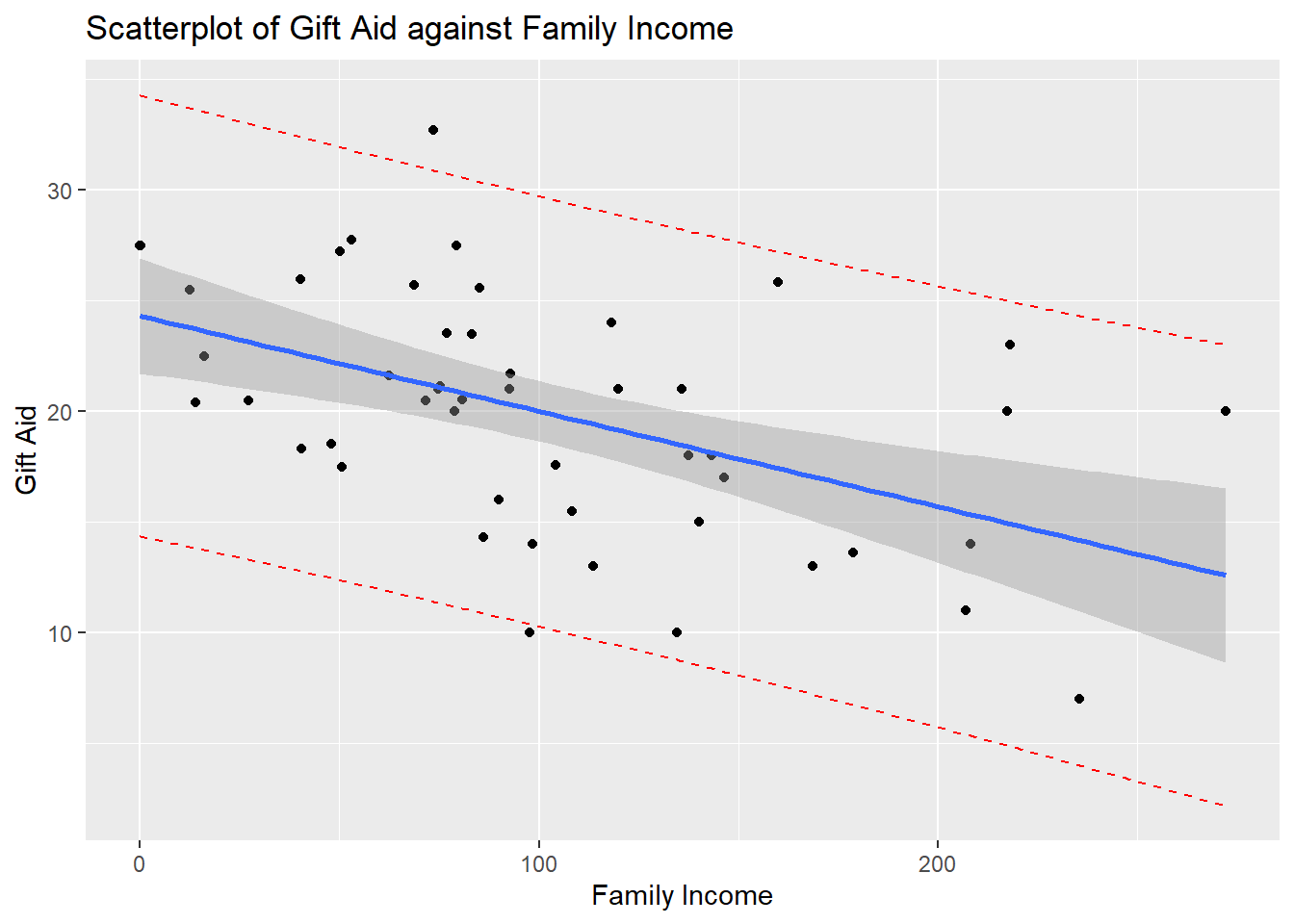

As mentioned in the notes, the CI captures the location of the regression line, whereas the PI captures the data points.

3 Basics with Simple Linear Regression (SLR)

5 Model Diagnostics and Remedial Measures in SLR

Linear Models for Data Science